


By Henry Peterson, Akshay Sridhar, Tapio Schneider, and Raffaele Ferrari
Part 13 of our tour of the CliMA software stack. The series began with why we built a new Earth system model; last week went from Hadley cells to atmospheric rivers.
Using the weather app on your phone or computer, you have likely noticed that atmospheric forecast models, like the one presented last week, cannot predict the weather more than a week or two in advance. This is a property of chaotic systems such as the atmosphere: beyond some finite time, the evolution of such systems cannot be predicted. How, then, can we predict the climate decades or centuries ahead? As we saw in part six of this series, climate is a statistical question, and the statistics of the weather are predictable when individual weather events are not. But there is a second question: why does the climate vary from year to year and decade to decade, when the weather that drives it has no memory beyond a couple of weeks? Klaus Hasselmann, who shared the 2021 Physics Nobel Prize with Syukuro Manabe (discussed in part four of this series) had the insight that the slow ocean accumulates the fast, random forcing of the weather, so that variability on long timescales emerges from the coupling itself. This week, we illustrate how coupling atmosphere, land, ocean, and sea-ice models (Figure 1) produces climate variability on timescales of years and beyond.
Coupling the entire CliMA software stack
In our tour of the CliMA software stack, we have encountered 14 stand-alone packages (Figure 2). Four of them, ClimaAtmos.jl, ClimaLand.jl, Oceananigans.jl, and ClimaSeaIce.jl, each represent one component of the climate system. Each can be run and tested in isolation and under various configurations. The final step is to couple them with ClimaCoupler.jl. The coupler has one job: to exchange fluxes of energy, water, and momentum between the components, conservatively. These three are the currencies traded among the components of the climate system, and the coupler exchanges only those. A hurricane blowing over the ocean imparts a wind stress curl at the surface, drawing cold subsurface water upward. The colder sea surface then reduces the latent heat flux to the atmosphere, which weakens the storm. While the physics of this communication is straightforward (the fluxes supply surface boundary conditions for each component), the mechanics are complicated in practice. How do you pass fluxes between models that live on different grids, take different time step sizes, and may run on different GPUs, while ensuring that the exchange of energy and water is conservative to floating-point precision?
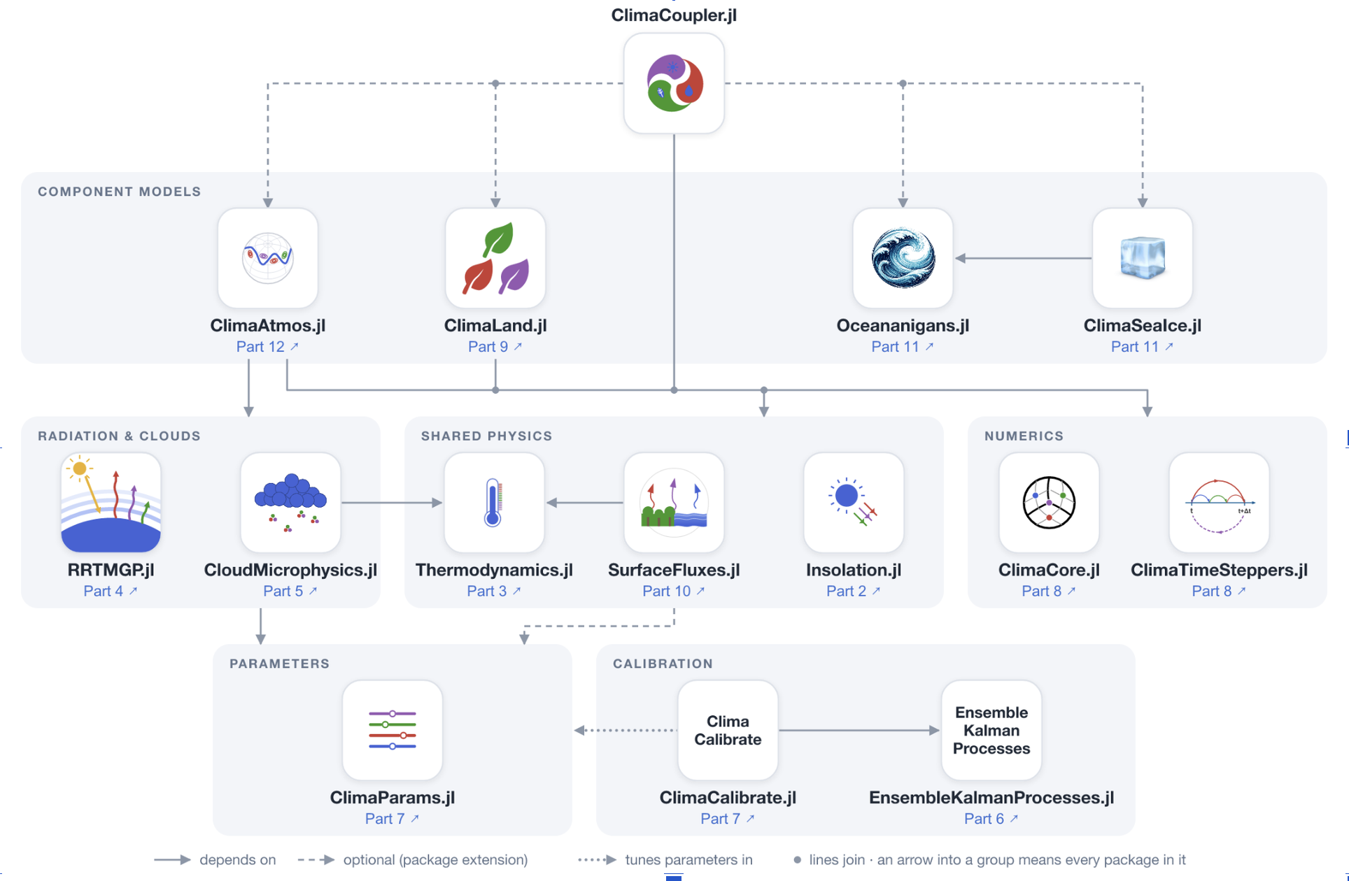
This is what ClimaCoupler.jl does, and it does so by drawing on the whole CliMA software stack. ClimaParams.jl provides the one set of parameters used across all models and ClimaCalibrate.jl the framework to calibrate them. Fluxes are computed with a consistent formulation using SurfaceFluxes.jl. Through the ClimaCore.jl extension in ConservativeRegridding.jl, variables are passed between the different model components conservatively: what the ocean receives at its surface is what the atmosphere sends. If, for instance, the ocean component can afford to take a time step larger than that of the atmosphere, the coupler accumulates fluxes from the atmosphere over one ocean step. It then sends the temporal average of these fluxes to the ocean, ensuring that water and energy are also conserved in time. The coupler interface is modular, allowing model components to be swapped depending on the application. By changing a configuration file, the ocean can go from a simple slab with a heat capacity to the full fluid solver of Oceananigans.jl with its parameterizations of turbulence. A new ocean model can be added through a Julia extension that implements the coupler interface. Because the entire CliMA software stack was built for GPUs, the coupled model runs on them as well.
A map of the net heat flux into the surface illustrates the many physical processes passing through the coupler at any given moment (Figure 3). The most obvious signal is the diurnal cycle of solar heating, sweeping around the globe every 24 hours. Over land, most of this radiation goes back into the air as sensible and latent heat, making it appear lighter on this color scale. The ocean, on the other hand, saturates the scale as it stores this heat over longer timescales. Places with cooler sea-surface temperatures, such as the equatorial cold tongue in the eastern Pacific, lose less heat at night and appear lighter. Clouds block some of the solar heating by day and trap outgoing longwave radiation at night. Sea ice loses heat at night in proportion to its concentration. In addition to this heating flux, the coupler passes fluxes of momentum, water, and more between the component models.
So what happens when we put all this together?
Coupled climate phenomena
El Niño has been in the news lately, with reports that this year’s could be the strongest on record. From these reports, you may already know the what, when, and how: every two to seven years, irregularly, the trade winds over the Pacific Ocean weaken, allowing warm water that is normally pooled on the western side of the basin to slosh eastward, with consequences for weather far away, such as extreme rain in California and severe droughts in Australia. Figure 4 shows this irregular oscillation in the equatorial Pacific sea-surface temperatures from a 30-year coarse run of ClimaCoupler.jl, the same kind of simulation you will run below.
But why does this happen? The ocean’s memory, in Hasselmann’s sense, is part of the story: as the atmosphere varies from week to week, the ocean responds slowly, and its slow response, controlled in part by the time it takes for temperature anomalies to cross the Pacific, sets the time scale of the oscillation. Another part is a feedback. If the trade winds weaken slightly, they allow warm water to shift eastward, deepening the eastern thermocline (the layer of rapid temperature changes below the mixed layer) and reducing the upwelling of cold water in the eastern Pacific. If the atmosphere felt no effect from the ocean, that would be the end of the story; instead, the resulting warmer sea surface in the east further weakens the trade winds, creating a reinforcing loop called the Bjerknes feedback. In the other phase, La Niña, the trade winds first strengthen, pushing more warm water west and driving stronger upwelling of cold water in the east; the sharper east–west temperature contrast strengthens the trade winds further. A model of the atmosphere alone or the ocean alone cannot produce these dynamics.

This two-way exchange is also at work on timescales of days to weeks. Two posts ago, we used ocean-only simulations to show why currents such as the Gulf Stream hug the western side of ocean basins. Much of that story was the surface wind forcing, the easterly trade winds in the tropics and the westerlies in the midlatitudes, visible in the last post’s animations. In our coupled simulations, as in observations, the Gulf Stream and the surface winds co-evolve (Figure 5). The Gulf Stream separates warm subtropical water from cold subpolar water, and the sharp temperature contrast across it helps steer the winds above, anchoring the storm track that runs along it. In turn, the winds drive the current through the momentum they transfer at the surface, forming a feedback loop. These coupled dynamics cannot be captured in ocean-only simulations with prescribed atmospheres.
While the sea ice appears stagnant on the one-week timescale of Figure 5, it grows and retreats over the seasonal cycle (Figure 1). Sea ice has a high albedo, reflecting around 10 times more solar radiation than the bare ocean. A warmer climate would cause the sea ice to melt and retreat, leading to more sunlight absorbed and more warming. Conversely, a cooler climate would lead to sea ice growth and further cooling. This ice–albedo feedback is present in the ClimaCoupler.jl simulations presented here, and it plays a critical role in variations of the coupled climate system over decades to millennia.
See for yourself
If you have followed the previous posts, you have run coarse versions of each component of the CliMA Earth system model on your own machine. Here, following the example in the documentation, we will put them together and run a coupled simulation for one year. A coupled climate model, even a coarse one, needs more than a laptop CPU: the run below (after installation and setup) takes about an hour to simulate one year on an NVIDIA GPU with 4 GB of memory or more.
First, start Julia in a fresh project with the GPU selected, from a terminal:
CLIMACOMMS_DEVICE=CUDA julia --project=coarse_cmip
Then install and load the packages (ClimaCore is pinned to the version the example was tested with):
using Pkg
Pkg.add(name = "ClimaCore", version = "1.0.5")
Pkg.add(["ClimaCoupler", "ClimaAtmos", "ClimaLand", "Oceananigans", "ClimaSeaIce", "ConservativeRegridding"])
Pkg.add(["ClimaComms", "CUDA"]) # For using an NVIDIA GPU
Pkg.add(["ClimaAnalysis", "CairoMakie"]) # For plotting

using ClimaCoupler

# The component models and the packages that load ClimaCoupler's extensions for them
import ClimaAtmos, ClimaLand, Oceananigans, ClimaSeaIce, ConservativeRegridding
import ClimaComms
ClimaComms.@import_required_backends
The simulation is specified by a configuration file. Load it, set the length of the run, and go:
config_file = joinpath(pkgdir(ClimaCoupler), "config", "longrun_configs", "cmip_coarse.yml")
config_dict = Input.get_coupler_config_dict(config_file)
config_dict["t_end"] = "365days"
cs = CoupledSimulation(config_dict)
run!(cs)
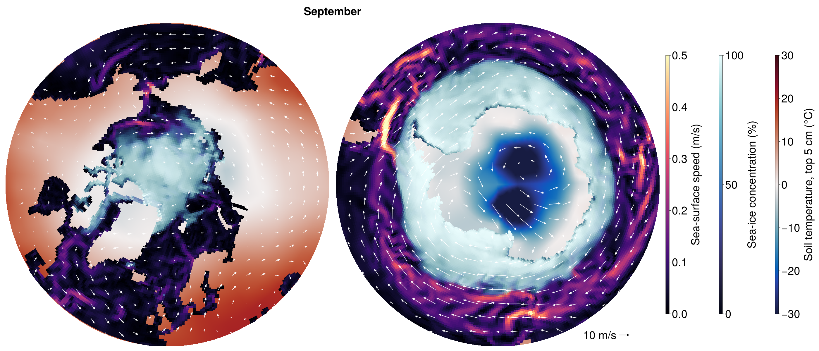
In this configuration, the horizontal resolution of the atmosphere and land is roughly 5° while that of the ocean and sea ice is roughly 1°. The atmosphere and ocean have 10 vertical levels each. At such a coarse resolution, without calibration, the model drifts over decades. (The Niño 3.4 index in Figure 4 was computed from detrended sea-surface temperatures.) The plotting code from the example in the documentation produces Figure 6 below.
This coarse simulation represents a minimal example that couples the four CliMA component models together. With more computational resources, higher-resolution setups with more sophisticated parameterizations are possible. ClimaCoupler.jl provides the tools necessary to ensure that all of these simulations achieve conservation to machine precision, and work is ongoing to use the framework described previously to calibrate the coupled model.
If you find the package useful, a star on the repository helps others discover it.
ClimaCoupler.jl is developed and maintained by the CliMA team with a growing team of external contributors.
Next week, a coda: what it took to build this, and what comes next.