

By Nat Efrat-Henrici and Tapio Schneider.
Part 7 of our tour of the CliMA software stack. The series began with why we built a new Earth system model; last week covered how to calibrate a model of a chaotic system.
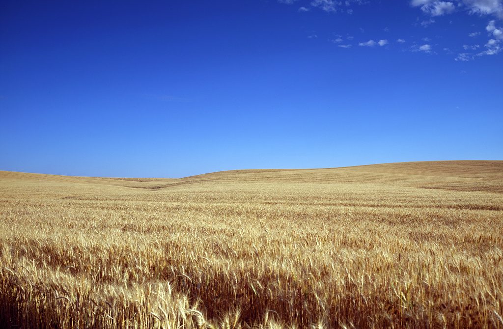
In the summer of 1968, a field campaign measured wind profiles over a field of wheat stubble in Kansas. Functional forms were fitted to those measured profiles, including a coefficient that sets how strongly stable temperature stratification damps turbulence near the ground. The fitted profiles with the coefficient, 4.7, have since been used to represent stable boundary layers in models worldwide, from the Great Plains to the Arctic, and they remain a mainstay in weather prediction and climate models today.
An Earth system model carries hundreds of such parameters, representing processes the model cannot resolve. Often they cannot be measured directly. From the perspective of calibration, a model that contains them is a black box: parameter values go in and climate statistics come out, with the statistics depending on the parameters, as we saw in the Lorenz model example in the previous post. The hundreds of thousands of lines of code and the physics they encode reduce to a forward map from parameters to output statistics. We learn the parameters by inverting the map: choose values, simulate, compare the output statistics to observations, update the parameters, iterate. This post is about the two packages that turn CliMA’s models into that map and inversion procedure: ClimaParams.jl, the single source of parameters, and ClimaCalibrate.jl, which iteratively inverts the map.
The art and science of tuning
For most of the history of climate modeling, parameters were tuned by hand. A 2017 survey found that 22 of 23 modeling centers adjusted parameters until the simulation looked right, yet the practice went largely undocumented, treated as “an unavoidable but dirty part of climate modeling,” leaving the process subjective and opaque. Until CMIP6, model intercomparisons did not ask for tuning to be documented at all.
The consequences affect the projections. Much of the spread between models in projected warming traces to cloud feedbacks, which are set by the parameterizations of clouds, convection, and boundary-layer turbulence, the very processes that were tuned by hand. A hand-tuned fit may not generalize out of today’s climate, and its uncertainty cannot be quantified: two wrong parameters can compensate for each other while reproducing today’s climate, or mask structural errors in the model. The compensation breaks under a forcing the model was not tuned against. Meanwhile, parameters lived wherever they were used, one value in a module of the atmosphere and a slightly different one for the same quantity in the land model, with the consequences for physical consistency we met in the thermodynamics post.
CliMA addresses each problem in turn. The scattered parameters are gathered into one package that every component model reads. And instead of being tuned by hand, they are calibrated by algorithms built for chaotic systems and noisy data, of the kind last week’s post described. Those algorithms need two things of a model: all adjustable parameters reachable from outside, and output comparable to observations. They accelerate model calibration and make it an objective, auditable process that becomes integral to development.
One source for all parameters
ClimaParams.jl provides one parameter set for CliMA’s atmosphere, land, ocean, thermodynamics, cloud microphysics, and radiation models. All entries carry descriptions with their units and, where known, their source. Since all model components read the same set, they use the same parameters. (The weights and biases of neural networks embedded in CliMA models are handled similarly, though they live in their own store.) A single line reaches far: gravitational acceleration has one entry, and it appears in the hydrostatic reference state, the fall speed of raindrops, the turbulence closure, surface fluxes, and in hydrostatic pressure reconstructions in radiation calculations.
Centralizing the parameters also makes the model portable across planetary configurations. The same microphysics scheme, given the gravity and fluid properties of another world, can produce the slow methane drops that fall on Titan, and the same lines compute the seasons of Mars. A planet is specified by parameter values rather than by hardcoded assumptions.
The Kansas wind profile coefficients live here too, used by SurfaceFluxes.jl, which computes the exchange of heat, momentum, and tracers such as CO2 with the surface for atmosphere, land, and ocean. Such parameters cannot be measured directly, only inferred from what the model produces. Such probabilistic inference starts from a statement of what is plausible. ClimaParams.jl holds that statement next to the value: together with a parameter’s value, units, and source, an entry can contain a prior distribution, in our illustrative example here, a constrained Gaussian with a mean of 3.0, a spread of 0.8, and hard bounds of 2 and 6.
constrained_gaussian("coefficient_a_m_businger", 3.0, 0.8, 2, 6)
Running the calibration
ClimaCalibrate.jl orchestrates the calibration: it runs the model for a parameter set to form an ensemble of simulations, collects the output, and hands the misfits to the algorithm for the next, data-adaptive update of the parameter set. To the calibration, a model run is just a map from a parameter set to output statistics that can be compared with observations. For CliMA models, the output statistics are aggregated during the simulation in the modules ClimaDiagnostics.jl and ClimaAnalysis.jl. Any model that can read a parameter file and produce output statistics can be calibrated in this way. The ensemble can run on whatever computing resources are available, whether that is a JuliaBackend() for a laptop or a DerechoBackend(...) for NCAR’s Derecho supercomputer, which we, like many academic groups, use extensively.
Calibration as part of a discovery loop
At CliMA, calibration is one node in an iterative, calibration-driven model development cycle. We calibrate weekly, sometimes several times a week, as a routine part of development. The misfit that remains once the parameter calibration has found a local optimum points to structural model errors: a process that is missing, or is represented in a way not fixable by adjusting parameters. This makes compensating and structural errors visible and actionable.
We use the residual errors in two ways. Where first-principles deduction allows, we improve the physics, which is the surest way to achieve out-of-distribution generalization: a residual in the stable boundary layer is a reason to revisit what a wheat field in 1968 can and cannot tell us about the Arctic. Where first-principles deduction reaches its limits, we embed expressive machine learning components that learn structural error corrections; the calibration machinery trains them. (The neural network that last week’s post fitted within a chaotic system was a version of this.) In both cases, the loop closes: calibrate, analyze the residual, modify the model, calibrate again. AI agents are beginning to take on parts of this loop, launching calibrations, diagnosing misfits, and proposing changes, in the direction of the automated knowledge discovery loop that a National Academies study described in 2022. The single source of parameters is what makes such a loop possible in the first place: an automated, iterative process requires transparent recording of its inputs.
See for yourself
ClimaCalibrate.jl provides an example calibration that runs SurfaceFluxes.jl on a laptop in seconds. We calibrate the wind profile coefficient against friction velocity, a measure of surface drag that flux towers measure routinely. This is a perfect-model test: the observation is produced as the model’s own output at the default parameter value of 4.7, with 1% noise added to mimic instrument error, and another 1% of model noise mimicking the internal variability that makes a climate model return a different statistic from run to run. We know the answer the calibration should recover.
import ClimaCalibrate
import EnsembleKalmanProcesses as EKP

# Defines observation, variance, prior, and SurfaceFluxModelInterface;
# the prior is constrained_gaussian("coefficient_a_m_businger", 3.0, 0.8, 2, 6)
include(joinpath(pkgdir(ClimaCalibrate), "experiments", "surface_fluxes_perfect_model", "utils.jl"))

# Unscented Kalman inversion: three members on a stencil around the mean
ekp = EKP.EnsembleKalmanProcess(observation, variance, EKP.Unscented(prior))

# Up to 15 iterations, on a swappable compute backend
ClimaCalibrate.calibrate(JuliaBackend(), ekp, SurfaceFluxModelInterface(output_dir, 3), 15, prior, output_dir)
Each iteration runs three forward models, and the calibration stops on its own once the misfit is down to the size of the noise.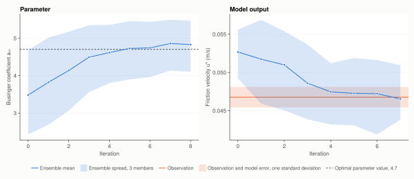
The parameter mean climbs from the prior and settles within about 0.1 of the true value, which is as close as the noise allows. The spread that remains, with this particular unscented Kalman inversion algorithm, quantifies the remaining uncertainty: it is an estimate of how well the noisy observation pins down the parameter. Hand tuning gives neither the number nor the uncertainty. Calibration gives both. The method scales from one parameter in a simple closure to hundreds in a full Earth system model.
If you find the packages useful, a star on the repositories, ClimaParams.jl and ClimaCalibrate.jl, helps others discover them.
ClimaParams.jl and ClimaCalibrate.jl are developed and maintained by the CliMA team; the full lists of contributors are on GitHub (ClimaParams, ClimaCalibrate).
The parameters now have a source and a way to be learned. Next week: the computational engine that puts models on a grid and steps them forward in time, with ClimaCore.jl and ClimaTimeSteppers.jl.