By Xin Kai Lee and Raffaele Ferrari

Part 11 of our tour of the CliMA software stack. The series began with why we built a new Earth system model; last week covered how the atmosphere exchanges heat, water, and momentum with the surface.

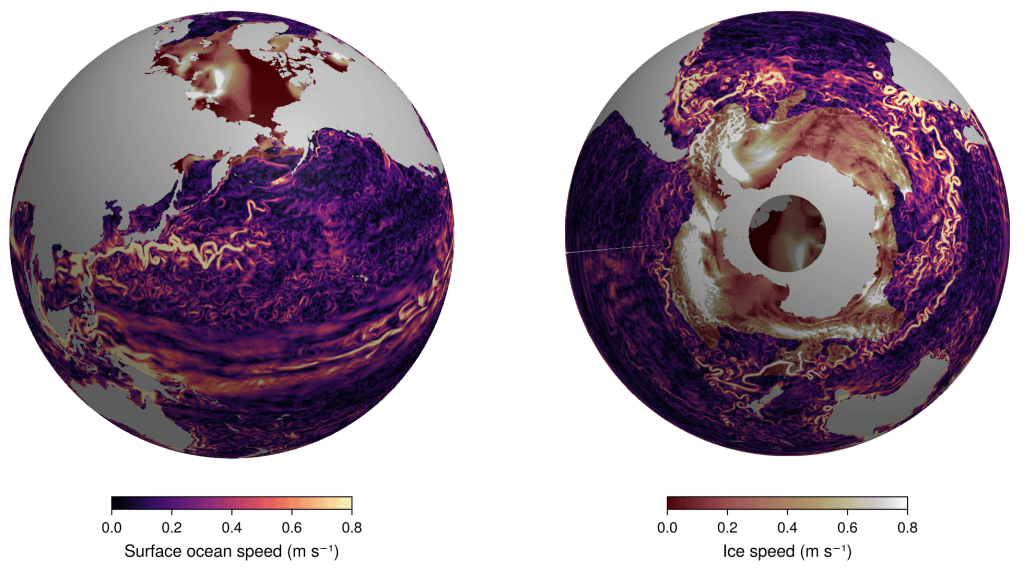
The ocean shapes Earth’s climate and weather. It is well known that the ocean absorbs about a quarter of our carbon dioxide emissions and most of the excess heat from global warming; other effects are less familiar. The climate of England and Portugal, for example, is much milder than that of the US coast at the same latitudes. Why? In this post, you will run global ocean simulations on your laptop, like the one used to make the video in Figure 1, and find an answer. The same model, but in a more realistic configuration, generated the image at the top of the post, showing the speed of surface water and sea ice.

Western boundary currents and climate

The story starts in the 1770s with Benjamin Franklin, who charted the Gulf Stream, a warm current flowing north along the US East Coast from Florida to North Carolina before turning eastward into the North Atlantic. It took until the 1940s for Henry Stommel, one of the founders of physical oceanography, to explain why such currents flow along the western sides of the ocean basins, that is, along the eastern margins of the continents: because Earth rotates and is a sphere. Oceanographers call them western boundary currents, after their position in the basins. They exist in all midlatitude basins: the Kuroshio along Japan, the Agulhas Current off South Africa, the Brazil Current along South America, and the East Australian Current.

You can now use Oceananigans.jl, the ocean component of the CliMA model, to see how Earth’s rotation and sphericity shape the ocean circulation and produce these currents. Oceananigans.jl is a library of solvers for the equations of fluid dynamics, written in Julia from scratch for GPUs. Silvestri et al. (2025) report 75 simulated years per day for a near-global ocean at a quarter of a degree on 16 NVIDIA A100 GPUs, and 10 years per day at 1/12 of a degree, about 8 km, on 64 GPUs. Those 64 GPUs fill 16 nodes of a current supercomputer, no more than the 10 to 300 nodes that CPU-based ocean models in climate projections use at resolutions of 25 to 50 km, where the ocean’s eddies have to be parameterized rather than resolved. Simulations are set up through a scripting interface, in two modes: non-hydrostatic, for high-resolution simulations of ocean turbulence down to meter scales, and hydrostatic, for regional simulations with open boundaries or for the global simulations of this post. The simulations in the tutorial run on a laptop, on its CPU or on an NVIDIA, AMD, or Apple GPU.

Now back to Stommel. Picture the ocean as an array of water columns, each reaching from the seafloor to the surface. Because each column rides on a spinning planet, it shares part of Earth’s spin (counterclockwise seen from above in the Northern Hemisphere), even when the water is perfectly still. At the poles, the column’s vertical axis lines up with Earth’s axis, and the column turns once a day. At the equator, the column is perpendicular to Earth’s axis and does not turn about its vertical at all. In between, the fraction of the Earth’s spin grows with latitude (technically, as the sine of latitude).

Winds set the water columns in motion. They blow from east to west in the tropics (the easterlies) and from west to east in midlatitudes (the westerlies). In the Northern Hemisphere, these winds exert a clockwise torque on the water columns between them, pulling them eastward on the poleward side and westward on the equatorward side. This torque opposes the columns’ counterclockwise spin, like a hand slowing a spinning wheel. On Earth, however, the columns can lose spin another way: by moving to lower latitudes, where the planet’s spin is weaker. So the water in the interior of the basin drifts toward the equator, and it has to return poleward somewhere, either up the eastern side of the basin or up the western side. Only one choice works. The wind keeps putting clockwise spin into the gyre, and friction has to remove it; a current along the western edge turns the gyre with the wind and lets friction take out the spin the wind puts in, whereas a current along the eastern edge would turn the gyre against the wind. The return flow of the entire basin is therefore squeezed into a narrow, fast current along the western edge. These currents are the Gulf Stream, the Kuroshio, and their cousins.

Stommel demonstrated this in 1948 with a simple model. On a flat Earth, where the spin does not depend on latitude, the gyre is symmetric, with no western intensification. On a spherical Earth, the return flow is concentrated along the western boundary, where friction removes the spin that the wind puts in. Western boundary currents are thus a consequence of Earth’s rotation, like the slow turning of Foucault’s pendulum in the Panthéon in Paris, and of its spherical shape. You can test this yourself in the tutorial by changing the planet’s rotation rate and sphericity.

At higher latitudes, the winds shift from westerlies to polar easterlies, and the torque on the ocean is counterclockwise. The interior flow is then poleward, and it is balanced by cold western boundary currents flowing toward the equator, such as the Labrador Current in the North Atlantic and the Oyashio in the North Pacific.

This brings us back to the mild winters of western Europe. The westerlies blow from the ocean onto Europe and from the continent onto the US East Coast, and the ocean, unlike land, stores summer heat and releases it in winter. That contrast between maritime and continental air does most of the work (Seager et al., 2002). The Gulf Stream and its extension add to it: the westerlies pick up additional heat as they cross these warm waters on their way to Europe. The current is part of the answer, and the rest of this post shows you how to simulate it.

Using Oceananigans.jl for global simulations

The tutorial sets up a global ocean simulation with realistic topography, one-degree horizontal resolution on a tripolar grid, and, to keep it fast, just four vertical levels, with a vertical coordinate that follows the free surface. The free surface is treated with a split-explicit scheme that subcycles the fast surface waves separately from the slow interior flow, and the advection uses high-order weighted essentially non-oscillatory (WENO) schemes, which increase the effective resolution at a given grid spacing. The ocean is forced with idealized wind and restoring to a surface-temperature pattern modeled on the observed zonal means. Convection, the sinking of cold water, cannot be simulated by a hydrostatic model and is represented by a simple convective adjustment scheme.

A simulation in Oceananigans.jl is a self-contained script. The blocks below sketch its structure; the full script, with the forcing, the output, and an experiment on the role of rotation and sphericity, is in the tutorial. The first step is to choose the hardware:

using Pkg; Pkg.add(["Oceananigans", "NCDatasets", "CUDA"])  # install once
using Oceananigans, NCDatasets, CUDA

arch = GPU() # No GPU? Remove `using CUDA` and use CPU().
             # AMD GPU: `using AMDGPU` and GPU(AMDGPU.ROCBackend()).
             # Apple silicon: `using Metal` and GPU(Metal.MetalBackend())

Next, download the topography, in this example, the ETOPO1 dataset, and interpolate it to the model grid, where it becomes an immersed boundary:

etopo_url = "https://www.ngdc.noaa.gov/thredds/dodsC/global/ETOPO1_Ice_g_gmt4.nc"
elevation = NCDataset(etopo_url) do dataset
    nomissing(dataset["z"][31:60:end, 31:60:end])
end

set!(elevation_field, elevation)
interpolate!(bottom_height, elevation_field)
grid = ImmersedBoundaryGrid(underlying_grid, GridFittedBottom(bottom_height, InterfaceImmersedCondition()); active_cells_map=true)

The boundary conditions include the wind stress at the surface, drag at the bottom, and a restoring of the surface temperature toward a prescribed pattern. Here is the temperature restoring:

# Surface temperature restoring
restoring_temperature(φ) = 30 * cos(deg2rad(φ))^2
temperature_flux(λ, φ, t, T, parameters) = parameters.rate * (T - restoring_temperature(φ))

temperature_restoring = FluxBoundaryCondition(temperature_flux; field_dependencies=:T, parameters=(; rate=restoring_rate))
T_boundary_conditions = FieldBoundaryConditions(top=temperature_restoring)

What remains is to choose the planetary rotation, the equation of state of seawater, the numerics, and the subgrid-scale closure, and to build and run the model:

coriolis = HydrostaticSphericalCoriolis(scheme=DualGridScheme(grid))
momentum_advection = WENOVectorInvariant(order=5)
tracer_advection = WENO(order=7)
buoyancy = SeawaterBuoyancy(equation_of_state=LinearEquationOfState(thermal_expansion=2e-4), constant_salinity=35)
closure = ConvectiveAdjustmentVerticalDiffusivity(convective_κz=1, convective_νz=1)

model = HydrostaticFreeSurfaceModel(grid; coriolis, buoyancy, closure,
                                    momentum_advection, tracer_advection,
                                    tracers = :T,
                                    timestepper = :SplitRungeKutta3,
                                    boundary_conditions = (u=u_boundary_conditions, v=v_boundary_conditions, T=T_boundary_conditions))

set!(model, T = (λ, φ, z) -> 10 * exp(z / 1000))
simulation = Simulation(model; Δt, stop_time=5year)
run!(simulation)

See for yourself

To run the simulation, download the full script from the tutorial and run it in a Julia session:

include("global_wind_driven_gyres.jl")

After a few simulated years, warm anomalies develop along the western boundaries. You can then change Earth’s rotation rate or its sphericity and watch the currents respond (Figure 2).

To go further, you can increase the horizontal or vertical resolution. For a realistic ocean, ClimaOcean.jl builds on Oceananigans.jl, adds forcing by winds, heat fluxes, and freshwater fluxes from atmospheric reanalysis, and couples the ocean to ClimaSeaIce.jl, which represents sea ice with a zero-layer thermodynamic model and an elastic–viscous–plastic rheology for its motion.

The tutorial configuration runs 1600 simulated years per day (SYPD) on one NVIDIA A100 GPU, and with 19 vertical levels, 1000 SYPD. That is the speed of an AI emulator: Samudra, which emulates a one-degree ocean model with 19 levels, ran about 1150 SYPD on one GPU when it was published, and its current version runs about 4800 SYPD. Emulators will be faster still at higher resolution, but they are trained on the output of a model and are reliable only near the states they were trained on; Samudra’s authors report that it struggles to reproduce the response to changing forcing, which is the response a climate model exists to compute. A model that solves the physical equations has no such restriction. The scaling of Oceananigans.jl to hundreds of GPUs is documented in Silvestri et al. (2025), and its numerics and interface in Wagner et al. (2025).

Our production simulations run at higher resolution. At a quarter of a degree, Oceananigans.jl simulates the strength and structure of the global overturning circulation without a parameterization of mesoscale eddies; matching the eddy kinetic energy observed from space takes 1/12 of a degree. In accuracy, this puts the CliMA ocean on par with established ocean models. In a future post, you will see Oceananigans.jl coupled to the atmosphere, land, and sea ice in a global Earth system simulation.

If you find the package useful, a star on the repository helps others discover it.

Oceananigans.jl was started at MIT by Ali Ramadhan, Simone Silvestri, and Gregory Wagner and is developed and maintained by the CliMA team with a growing team of external contributors.

Next week: the atmosphere, from Hadley cells to atmospheric rivers, with ClimaAtmos.jl.