Part 5 of our tour of the CliMA software stack. The series began with why we built a new Earth system model; last week covered radiative transfer, a Nobel-winning calculation, runnable in minutes.

The total water vapor in Earth’s atmosphere, if it all rained out, would cover the globe with a liquid layer on average only about 22 mm (less than an inch) deep. We cannot see this water vapor in the air. It only becomes visible once it condenses into liquid droplets or ice crystals. Whenever we see a white cumulus cloud on a summer day, a thunderstorm anvil in the afternoon, or a patch of fog on a cold morning, we are looking at millions of small water particles suspended in the air. How many? A typical cloud holds about 100 droplets per cubic centimeter, which for a modest cloud, one kilometer on each side, comes to a hundred quadrillion droplets. Yet with each droplet only about 10 micrometers in radius, that cloud is 99.99996% empty space by volume. If you are curious what it weighs anyway, Karen LaMonte’s sculpture “Cumulus” in the image at the top, carved in marble based on our simulations, weighs about as much as the condensed water in a fair-weather cumulus cloud.

Here is the puzzle those numbers add up to. A raindrop, with a millimeter radius, contains the water of about a million cloud droplets. But droplets grow by condensation more and more slowly as they get bigger: growing from 10 to 11 micrometers takes about five minutes, and from 16 to 17 micrometers about half an hour. At that rate, condensation alone would need days to produce drizzle. Yet a growing cumulus can rain twenty minutes after forming. By the arithmetic of condensation, rain should barely exist. It does anyway, so something else must take over when condensation stalls.

From droplets to raindrops

What takes over is collisions. In warm (liquid) clouds, after initial condensational growth, it is the collisions and coalescence of cloud droplets buffeted by turbulence that lead to the formation of drizzle and rain: a falling drop sweeps up the smaller droplets in its path, and its growth accelerates. The same growth explains why clouds do not fall out of the sky. Cloud particles are small and light enough that turbulent updrafts keep them suspended; only once collisions have grown a particle such that its fall speed exceeds the rising air around it does it precipitate. In colder clouds, ice crystals steal water vapor from droplets, and, depending on surrounding conditions, the ice can grow into beautiful snowflakes or clump and aggregate into graupel or hail.

The droplets themselves also need help to exist. There is not enough water vapor in the atmosphere to form cloud droplets and ice crystals unaided: aerosol particles (very small particles of dust, sea salt, etc.) have to be present to serve as condensation nuclei for both. You can see it for yourself in this video from the Arctic: mist does not form over a hot cup of tea in pristine Arctic air until smoke from a lighter provides condensation nuclei.

All of this plays out on scales of micrometers. The quantity to be predicted is minuscule: while all the water vapor in the atmosphere amounts to a 22 mm liquid layer, all the condensed water in clouds, liquid and ice together, amounts to a layer covering the globe only 0.1 mm deep, roughly the thickness of a human hair. Cloud microphysics must predict the fate of the tiny condensed fraction of a trace constituent of the atmosphere, on scales no climate model will resolve in the foreseeable future. Representing what these processes do to the planet is the job of the CliMA package CloudMicrophysics.jl.

Why it matters for climate

We are used to hearing about trace gases such as carbon dioxide and methane that warm our planet. Some of that warming, however, is masked by the cooling effect of pollution: aerosol particles reflect solar radiation back to space. As we clean up aerosol pollution, we save lives by improving air quality, but we also remove some of the masking that has been slowing the warming. The number and type of aerosol particles also set how many cloud droplets and ice crystals form, which in turn affects how long clouds last, how much sunlight they reflect, and how readily they precipitate. To predict how much warming emerges as the air gets cleaner, a model must trace the causal chain from aerosol counts, through the populations of droplets and crystals and their microphysical behavior, to the cloud optical properties that enter the radiative transfer calculations we met last week. Correlations learned from today’s polluted atmosphere cannot extrapolate to a cleaner one; the causal chain can.

One package for the unresolvable

CloudMicrophysics.jl is a library of parameterizations: building blocks that anyone can use to assemble their own cloud model. The blocks form a hierarchy of complexity. At the base are zero-moment schemes, which track no condensed water at all; the model rains directly out of the vapor, without regard for cloud water, a simplification that was common in climate models until fairly recently. One-moment schemes track the masses of cloud water and ice. Two-moment schemes additionally track number concentrations, so a cloud of many small droplets can be told apart from a cloud of few large ones, which is the distinction on which the aerosol effects above hinge. And modern schemes such as P3 let the properties of ice particles evolve continuously instead of tracking fixed categories such as snow and graupel.

Some parameterizations rely on simple physical assumptions, letting users spin up simulations quickly and calibrate unknown parameters against data; others are grounded in recent large-scale field or laboratory measurements and may need less calibration. The package is modular, so parameterizations can be mixed and matched. All of them run on GPUs, are differentiable, and draw their thermodynamics from Thermodynamics.jl, for consistency with the rest of the stack. No free parameter is hard-coded, which makes the package ready for the data-driven calibration we turn to next week. The same building blocks can be used in configurations ranging from the simple parcel model we use in our documentation to CliMA’s full weather prediction and climate model. And because we kept the physics invariant wherever possible, the building blocks can be used broadly; for example, changing planetary parameters such as the gravitational acceleration can produce the slowly falling methane raindrops of Titan that we encountered two posts ago.

See for yourself

The full documentation offers many usage examples, along with brief derivations of the theory behind each library component. Here we reproduce one of the tutorials and make rain in under twenty minutes of simulated time.

We import the packages we need: an ordinary differential equation solver and a plotting package from the Julia ecosystem, and the cloud microphysics modules. We define the model, with two processes converting cloud water to rain: autoconversion (collisions among cloud droplets that form the first raindrops) and accretion (falling raindrops collecting the cloud droplets in their path).

import OrdinaryDiffEqTsit5 as ODE
import CairoMakie as PLT

import CloudMicrophysics.Parameters as PRM
import CloudMicrophysics.Microphysics1M as CM1
import CloudMicrophysics.ThermodynamicsInterface as TDI

function rain_formation(dY, Y, p, t)
    FT = eltype(Y) # Floating point precision type
    (; mp, tps, ρₐ, T) = p # Additional parameters passed through p

    qₗ = Y[1] # Cloud water specific content
    qᵣ = Y[2] # Rain water specific content

    # Construct the state tuples expected by the option-dispatched API
    micro = (; q_tot = qₗ + qᵣ, q_lcl = qₗ, q_icl = FT(0), q_rai = qᵣ, q_sno = FT(0))
    thermo = (; ρ = ρₐ, T = T)

    procs = mp.processes
    acnv = CM1.conv_q_lcl_to_q_rai(procs.rain_autoconversion, mp, tps, micro, thermo)
    accr = CM1.accretion(procs.cloud_liquid_rain_accretion, mp, tps, micro, thermo)

    dY[1] = -acnv - accr # Add the tendencies for cloud water
    dY[2] = acnv + accr  # and rain
end

All parameter values come from the package defaults. No source code of the library needs to be touched.

FT = Float32

mp = PRM.Microphysics1MParams(FT) # 1-moment microphysics parameters (includes options)
tps = TDI.TD.Parameters.ThermodynamicsParameters(FT) # Thermodynamics parameters
ρₐ = FT(1) # Air density
T = FT(280) # Temperature (unused by warm-rain processes, but required by the API)
p = (; mp, tps, ρₐ, T)

t₀ = FT(0)
t_end = FT(10 * 60)
TS = (t₀, t_end)

qₗ0 = FT(5e-3)
qᵣ0 = FT(0)
IC = [FT(qₗ0), FT(qᵣ0)]

problem = ODE.ODEProblem(rain_formation, IC, TS, p)
sol = ODE.solve(problem, ODE.Tsit5(), reltol = eps(FT), abstol = eps(FT))

fig, ax, _ = PLT.lines(sol.t, sol[1, :] .* 1e3; label = "cloud")
PLT.lines!(ax, sol.t, sol[2, :] .* 1e3; label = "rain")
ax.xlabel = "time [s]"
ax.ylabel = "q [g/kg]"
PLT.axislegend(ax; position = :rc, framevisible = false)
PLT.save("rain_formation.png", fig)

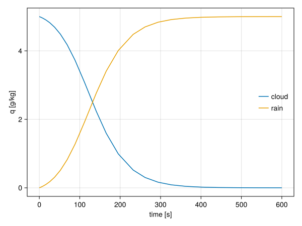
The figure below shows the result: cloud water drains away as rain grows, and most of the conversion happens within minutes once accretion takes hold; collisional growth takes over when condensation stalls.

If you find the package useful, a star on the repository helps others discover it.

CloudMicrophysics.jl is developed and maintained by the CliMA team; the full list of contributors is on GitHub.

Next week: no one can predict the weather a month ahead, yet we can calibrate climate models against chaos, with EnsembleKalmanProcesses.jl.