

By Zhaoyi Shen and Tapio Schneider.
Part 4 of our tour of the CliMA software stack. The series began with why we built a new Earth system model; last week covered methane rain on Titan and the thermodynamics of moist air.
Water vapor is the most important greenhouse gas on Earth. Removing all water vapor from an atmospheric column in a one-dimensional climate model cools the surface by 24 K, to well below freezing; removing the CO2 instead cools the surface by 17 K. Yet we do not track water vapor emissions, because water vapor provides a feedback, not a forcing. Its concentration is controlled primarily by temperature (roughly 7% more vapor per degree of warming, as we saw last week). If CO2 rises, water vapor roughly doubles the temperature response.
How do we know the answers to such counterfactual questions? Inductive inference from data alone does not suffice. It must be paired with the deductive power of physical calculations.
Manabe’s deduction
In the 1960s, Syukuro “Suki” Manabe and his collaborators built the first Radiative-Convective Equilibrium (RCE) model: a single column of atmosphere in which detailed spectral calculations of solar and infrared radiation balance a simple convective adjustment. Manabe’s brilliant insight was to fix the relative humidity of the atmosphere, so that the amount of water vapor rises and falls with temperature. That assumption, since broadly confirmed by theory and decades of data, embeds water vapor feedback in RCE calculations.
The model made predictions that were deduced from physics. It predicted roughly 2.0 K to 3.0 K surface warming from doubling CO2. It predicted that while the surface and troposphere warm, the stratosphere cools—a telltale fingerprint of greenhouse warming that was observed decades later. The model yielded the first credible estimate of Earth’s climate sensitivity and laid the groundwork for modern climate modeling. For this work, Manabe shared the 2021 Nobel Prize in Physics.
The radiation code
For the CliMA ecosystem, RRTMGP.jl provides high-fidelity radiative transfer. It computes radiative fluxes and heating rates for clear, cloudy, and aerosol-laden atmospheres, and also provides an analytic gray-radiation mode for idealized studies, so a user can move through a hierarchy of configurations, from textbook problems to state-of-the-art spectral calculations. The package is derived from RTE+RRTMGP, developed by Robert Pincus, Eli Mlawer, and Jennifer Delamere as the modern successor to RRTMG, a widely used radiation scheme. We rewrote it in Julia, and the same code now runs on CPUs and GPUs, in single or double floating-point precision.
The rewrite went beyond translation. Historically, radiation codes have struggled to run in single precision (Float32) because optically thin atmospheric layers and near-singular two-stream formulas lead to catastrophic cancellation when nearly equal numbers are subtracted. RRTMGP.jl solves this by rewriting the underlying math to be more robust to roundoff error. By reducing cancellation errors, the Float32 results become virtually identical to Float64, with longwave fluxes now agreeing to within a few times 10-4 W/m2. Running in Float32 halves the memory traffic, now without sacrificing accuracy; the improvements can flow back to the upstream code from which RRTMGP.jl was derived.
Using single-precision arithmetic and tailoring its memory layout to GPU hardware, RRTMGP.jl achieves large GPU acceleration. On a benchmark typical for atmosphere models (86,400 columns, 63 layers), an NVIDIA A100 GPU completes a full clear-sky radiation step 84× faster than a 12-thread Intel CPU. Translating this performance into standard AWS cloud compute pricing, running a radiation step on a GPU is more than 10 times cheaper than on a multi-threaded CPU, making climate modeling more broadly accessible. Additionally, a GPU consumes roughly 50 times less total electricity to compute the same physics, lowering the carbon footprint of our climate simulations. These accelerations for radiative transfer are typical of what we see across the CliMA modeling stack.
| Configuration | CPU Intel Xeon, 12 threads |
GPU NVIDIA A100 40GB |
Speedup |
|---|---|---|---|
| Clear-sky | 80.05 s | 0.95 s | 84.3× |
| All-sky | 99.44 s | 1.40 s | 71.0× |
| All-sky with aerosols | 106.77 s | 1.56 s | 68.4× |
Why the physics stays
Radiation also provides a clear illustration of why we build a physical scaffolding for the CliMA model, rather than trying to learn everything from data. Machine learning excels where the future that needs to be predicted resembles the available training data, as in weather forecasting. But the response of the climate system to unseen CO2 concentrations cannot be learned from observations alone; it must be deduced from spectroscopy measured in laboratories and radiative transfer derived from first principles. The stratospheric cooling Manabe predicted was such a deduction, made decades before it was observed. So in CliMA, we keep physics where we can and learn from data where deduction from first principles reaches its limits (for example, snow, clouds, and turbulence, in later posts). In radiative transfer, ML can help compress spectroscopic data, but physics is required to compute how radiation propagates through the atmosphere.
See for yourself
Recreating Manabe’s classic experiments is straightforward in RRTMGP.jl. A runnable RCE tutorial is in the RRTMGP.jl documentation. The tutorial shows how to toggle between radiative and radiative-convective equilibrium, switch between fixed absolute and relative humidity, adjust greenhouse gas concentrations, and modify the convective lapse rate.
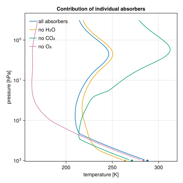
The figure below highlights RCE results for individual absorbers. When all greenhouse gases are included, the model reproduces a temperature profile close to Earth’s: a troposphere convectively coupled to the surface, a tropopause near 200 hPa (11 km), and a stable stratosphere above. Removing one gas at a time, their relative effects become clear: water vapor provides the largest greenhouse warming (removing it cools the surface by 24 K), followed by CO2 (17 K). Ozone controls the temperature structure of the upper atmosphere by warming the stratosphere.
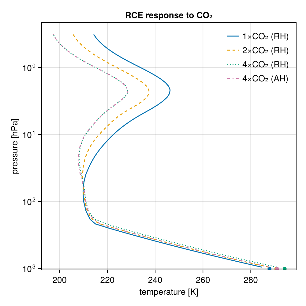
The figure at the top illustrates the RCE response to increasing CO2 concentrations. Doubling CO2 raises the surface temperature by 2.9 K, while quadrupling it yields a 6.3 K increase. This demonstrates that the warming is roughly logarithmic with respect to CO2 concentrations. The model also captures the strong cooling of the stratosphere as CO2 levels rise. By comparing these results against a fixed absolute humidity run (3.1 K surface warming for 4×CO2 ), we can quantify the water vapor feedback: it approximately doubles the surface warming driven by CO2 alone.
If you find the package useful, a star on the repository helps others discover it.
RRTMGP.jl is developed and maintained by the CliMA team, building on RTE+RRTMGP and its Fortran implementation by Robert Pincus, Eli Mlawer, and Jennifer Delamere; the full list of contributors is on GitHub.
Next week: how cloud droplets grow up to become raindrops, with CloudMicrophysics.jl.