Part 8 of our tour of the CliMA software stack. The series began with why we built a new Earth system model; last week covered how we learn a climate model’s parameters from data.

Simulating a physical system in space and time requires a discretization: a grid in four-dimensional space-time, on whose nodes we predict, in the case of the atmosphere, temperatures, winds, humidity, rainfall, and other variables. CliMA’s discretization is split across two packages. ClimaCore.jl handles space; ClimaTimeSteppers.jl handles time.

Four requirements shaped their design:

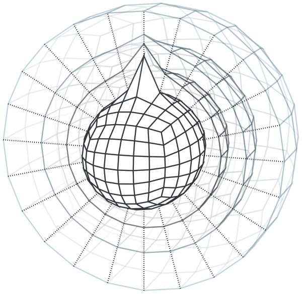
• The globe must be tiled into elements of roughly equal size, so that all of them can be stepped forward in time by the same amount. Ordinary latitude-longitude grids don’t satisfy this, as their cells are squeezed to points at the poles, and the smallest cell dictates the time step for the whole globe. The cubed sphere grid, shown in Figure 1, does better. It projects the six faces of a cube onto the globe and lays a rectangular grid on each face.
• Only a thin shell of the globe matters for climate: the atmosphere (primarily the troposphere and stratosphere), the ocean, and the upper layers of the land surface. If Earth were shrunk to the size of an apple, the troposphere and stratosphere would be about as thick as the apple’s skin. On a typical grid with 25–100 km horizontal spacing, with cells near the ground that are tens of meters tall (an aspect ratio near 1000:1), vertical operations must be discretized differently from horizontal ones.
• The same code base should run cloud-resolving simulations in a box and global climate simulations on a sphere. With scale-dependent parameterizations, one set of discretized equations can be used to simulate vastly different scales of atmosphere, ocean, or land.
• Extensive quantities such as energy and total water must be conserved to round-off error. Climate models run for millions of time steps, over which even minuscule errors would cause the simulation to drift away from a realistic climate.

Putting the model on a grid

ClimaCore.jl provides the mathematical operators through which ClimaAtmos.jl and ClimaLand.jl express their differential equations. Variables are defined as fields over a spatial grid, and can be manipulated with standard mathematical functions (sums, logarithms, etc.) or with the differential operators of vector calculus (gradient, divergence, and curl).

Behind the scenes, the fields live on a bounded domain—a line for a vertical column, a box for a large-eddy simulation, or a spherical shell for a full global model. The domains are discretized with finite differences in the vertical and spectral elements in the horizontal. Each spectral element represents a field within a quadrilateral patch of the grid by the nodal values of a high-order polynomial, and each vertical cell stores variables on either cell faces or cell centers. We store vertical velocity on cell faces and all other fields at cell centers, which avoids spurious “computational modes” that unstaggered grids generate and that can produce noise (Thuburn and Woollings, 2005). The grids are optimized for the atmosphere’s aspect ratio. Small vertical spacing requires tight coupling between the points in each column; the large horizontal spacing allows computing each spectral element in parallel, with dense local arithmetic that performs well on GPUs.

Spatial fields are stored as arrays whose entries correspond to points on the grid. As shown in Figure 1, grids incorporate topography through terrain-following coordinates, and the differential operators account for the resulting curvature of the grid to simulate flow over mountains.

Two numerics, one model

The spectral element method comes in two flavors, which differ in how neighboring elements are coupled. Continuous Galerkin (CG) enforces continuity across element boundaries by averaging the values that horizontally neighboring elements compute at their shared nodes. Discontinuous Galerkin (DG) lets the values differ and couples the elements through horizontal numerical fluxes across their interfaces. Both conserve mass and tracers to floating-point precision. CG is the established choice, used by the dynamical cores of the NCAR and DOE climate models. It is the simpler of the two computationally, but it requires artificial damping (“hyperdiffusion”) to remove grid-scale noise the discretization generates. DG instead obtains its dissipation from the interface fluxes, as in upwind-biased finite-volume methods, and needs no artificial damping. It combines the high-order accuracy and element-local structure of spectral methods with the robustness of finite-volume methods.

ClimaCore can run CG and DG from the same model code. Either method computes tendencies (rates of change of state variables) elementwise. This leaves the results incomplete at element boundaries, where each element only has information about its own side. A call to complete_tendency! finishes a tendency calculation in whichever way the method demands: by averaging the shared nodes on a CG grid, or by adding the interface fluxes on a DG grid. The Bickley jet tutorial demonstrates this for the shallow-water equations. A keyword argument is used to switch between CG and DG when constructing a grid:

cg_space = Spaces.SpectralElementSpace2D(topology, quad; discretization = Grids.CG())
dg_space = Spaces.SpectralElementSpace2D(topology, quad; discretization = Grids.DG())

The tendency, written with the vector-calculus operators used in textbooks and papers, is the same function on either grid:

function shallow_water_rhs!(dydt, y, (p, completion), t)
    wdiv = Operators.Divergence{Operators.WeakForm}()
    @. dydt = -wdiv(sw_flux(y, (p,)))                     # element-local weak divergence of the flux
    Operators.complete_tendency!(completion, dydt, y, p)  # DSS on CG, interface fluxes on DG
    return dydt
end

completion = Operators.tendency_completion(dydt; numflux)  # chosen by the space: DSS or numerical flux

Stepping forward in time

ClimaCore discretizes space; ClimaTimeSteppers.jl advances the discrete equations in time. The grid’s aspect ratio dictates the design here too. An explicit time stepper is stable only if no signal travels farther than about one grid cell per step. In the compressible equations solved by ClimaAtmos, the fastest signals are sound waves, traveling at about 300 m/s. At 30 km horizontal resolution, a sound wave needs about 100 seconds to cross a cell horizontally. Near the surface, where cells are tens of meters tall, it needs only about 0.1 seconds to traverse the cell vertically. A fully explicit model therefore would need steps of about 0.1 seconds, or some 10¹⁰ steps per simulated century, to track waves that carry no climate signal. Yet sound waves matter to a climate model because they communicate pressure changes across the globe, so a time stepper must handle them stably.

The remedy is to split the tendency into two parts:

• The vertical operations that generate fast signals go into an implicit tendency: acoustic and gravity waves in ClimaAtmos, the rapid vertical diffusion of water and energy in ClimaLand, and, optionally, precipitation and vertical diffusion in the atmosphere. Instead of tracking these signals step by step, the implicit tendency is applied by solving a boundary value problem in each column. The solve uses Newton’s method, in which each iteration solves a linear system built from the Jacobian of the implicit tendency (its derivative with respect to the state variables); ClimaCore’s matrix-field solver does so efficiently as a chain of tridiagonal solves and matrix-vector products.
• Everything else, including horizontal acoustic and gravity waves, radiation, and the other slower processes, forms an explicit tendency. The step size is then limited by the fastest horizontal waves: at resolutions of 50–200 km, ClimaAtmos takes steps of several hundred seconds, thousands of times longer than the vertical sound waves would otherwise allow.

ClimaTimeSteppers provides a collection of well-tested schemes for this splitting: additive Runge-Kutta implicit-explicit (IMEX) methods, multirate methods that substep the fast processes, and Rosenbrock methods that linearize the implicit part. All of them take ClimaCore fields as their state vectors, so they can step forward in time what ClimaCore discretizes in space.

Performance across devices

ClimaCore’s operators are built from a small set of parallelization primitives, each implemented for CPUs and for GPUs, with distribution across compute nodes through MPI. The primitives are loops over slices of the domain (elements, columns, or points), reductions across points, specialized linear solvers, and the inter-element communication of the two discretizations (averaging of shared nodes for CG, numerical fluxes for DG). Everything built on top of the primitives is device-independent, with the same code executing on both CPUs and GPUs. On GPUs, the cost of a time step is often set by the number of kernels launched and the memory traffic each incurs rather than by arithmetic, so operators that act along the same direction can be fused into larger kernels, either by combining them into longer expressions, or by wrapping them in a loop over points (foreach_point), columns (foreach_column), or other slices of the domain.

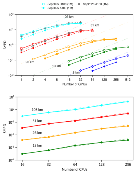
The result is throughput competitive with leading GPU-based atmosphere models. Given a few dozen GPUs, ClimaAtmos runs at more than one simulated year per day (SYPD) with 25–50 km horizontal resolution (Yatunin et al., 2026). Weak scaling efficiency exceeds 92% on GPUs and 98% on CPUs, so adding processors for a larger problem preserves efficiency. Strong scaling—adding GPUs to a fixed-size problem—is over 95% efficient as long as each GPU holds at least about 5,400 spectral elements; below that, kernel launch and communication overheads dominate. The throughput is comparable to that of other leading GPU atmosphere models, and the time per step is nearly an order of magnitude shorter than that of Pace, the only other nonhydrostatic atmosphere model written in a high-level language. GPUs also make high-resolution simulation accessible well beyond supercomputing centers. A few dozen cloud GPUs, available to many research groups, suffice for the atmosphere at 25–50 km resolution at more than one simulated year per day (SYPD); the land model, built on the same ClimaCore operators, runs at around 100 SYPD on a few GPUs (Deck et al., 2026).

See for yourself

ClimaCore.jl offers tutorials ranging from a single-column PDE to a three-dimensional cubed sphere. For the latter, constructing the discretization takes a few lines: a vertical grid, a horizontal grid, and their product.

radius = 6e6   # 6000 km
height = 1e3   # 1 km
device = ClimaComms.device()

# Vertical: a staggered finite-difference column of 10 levels
vert_domain = Domains.IntervalDomain(Geometry.ZPoint(0.0), Geometry.ZPoint(height); boundary_names = (:bottom, :top))
vert_mesh = Meshes.IntervalMesh(vert_domain; nelems = 10)
vert_space = Spaces.FaceFiniteDifferenceSpace(device, vert_mesh)

# Horizontal: a cubed sphere with 10 × 10 spectral elements per face, cubic polynomials
horz_domain = Domains.SphereDomain(radius)
horz_mesh = Meshes.EquiangularCubedSphere(horz_domain, 10)
horz_topology = Topologies.Topology2D(ClimaComms.context(device), horz_mesh)
horz_space = Spaces.SpectralElementSpace2D(horz_topology, Quadratures.GLL{4}())

# The three-dimensional space is the product of the two
space = Spaces.ExtrudedFiniteDifferenceSpace(horz_space, vert_space)

FaceExtrudedFiniteDifferenceSpace:
  horizontal:
    mesh: 10×10×6-element EquiangularCubedSphere of SphereDomain: radius = 6.0e6
    quadrature: 4-point Gauss-Legendre-Lobatto quadrature
  vertical:
    mesh: 10-element IntervalMesh of IntervalDomain: z ∈ [0.0,1000.0] (:bottom, :top)

Once the space is defined, operations on fields are written as broadcast expressions, which compile to a loop on a CPU or a kernel on a GPU, depending on where device points:

(; lat, long, z) = Fields.coordinate_field(space)
blob = @. exp(-(lat^2 + long^2) / 15^2) * (z < 5)   # a Gaussian blob near the surface

Swapping SphereDomain for a periodic RectangleDomain converts the spherical simulation into a periodic box; dropping the horizontal space gives a single-column simulation, which we use regularly for testing parameterizations.

The four requirements we began with are met by construction. The cubed sphere tiles the globe into elements of roughly equal size. The extruded space combines vertical columns on a staggered grid with an element-local horizontal grid, respecting the atmosphere’s aspect ratio. The domain is a keyword, so the same code can be run in a box or on the globe by changing that keyword. Finally, the operators on the selected space conserve mass and tracers to round-off, and energy is also conserved provided it is used as a prognostic variable, as is done in ClimaAtmos and ClimaLand. All simulations written with this interface are agnostic about running on a laptop or on hundreds of GPUs.

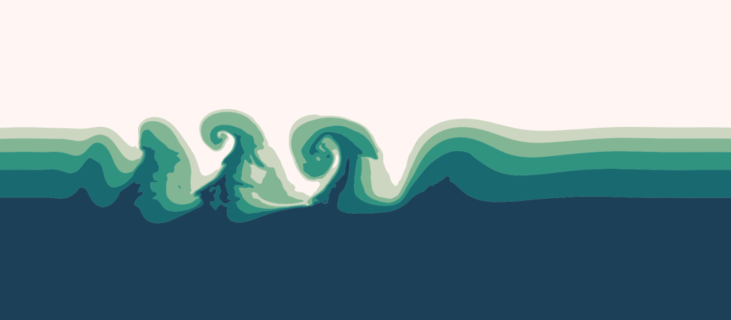
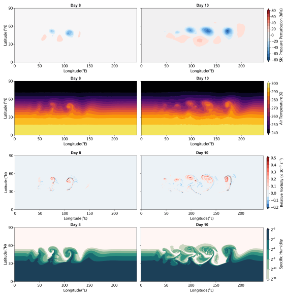
For examples with the full set of differential operators and time integration, see the documentation. One of the more complex examples is the baroclinic wave benchmark simulation, whose moist version is shown in Figure 3 and at the top of the post.

If you find the packages useful, a star on the repositories, ClimaCore.jl and ClimaTimeSteppers.jl, helps others discover them.

ClimaCore.jl and ClimaTimeSteppers.jl are developed and maintained by the CliMA team; the full lists of contributors are on GitHub (ClimaCore, ClimaTimeSteppers).

Next week: why you cannot get the dust off your car by driving fast, with SurfaceFluxes.jl an intermezzo laying out the reasoning behind how we use AI at CliMA, prompted by the Navier-Stokes Millennium Prize discussions.