By Julian Schmitt and Tapio Schneider

Everything in the climate system begins with sunlight. Weather, ocean currents, and the growth of forests are all powered by solar radiation entering at the top of the atmosphere. The amount arriving at any particular place and time is the insolation: the solar power passing through a unit area tangential to the top of the atmosphere. Insolation is a function of the solar radiative energy flux, which varies with the Earth–Sun distance, and the elevation of the Sun in the sky, which varies with location, time of day, and time of year. Aside from small variations in solar output (roughly 0.1% over the 11-year sunspot cycle, or about 1 W/m² in total solar irradiance), all variations in insolation are geometric, inherited from Kepler and Newton, and can be calculated to almost any precision desired.

For our Earth system model, we calculate insolation with the CliMA package Insolation.jl: for Earth right now in our weather model configuration, for Earth at any time in the past 50 million years or the next 20 million in climate simulations, and, by specifying a handful of orbital and solar parameters, for any planet in a low-eccentricity orbit.

The strange geometry of sunlight

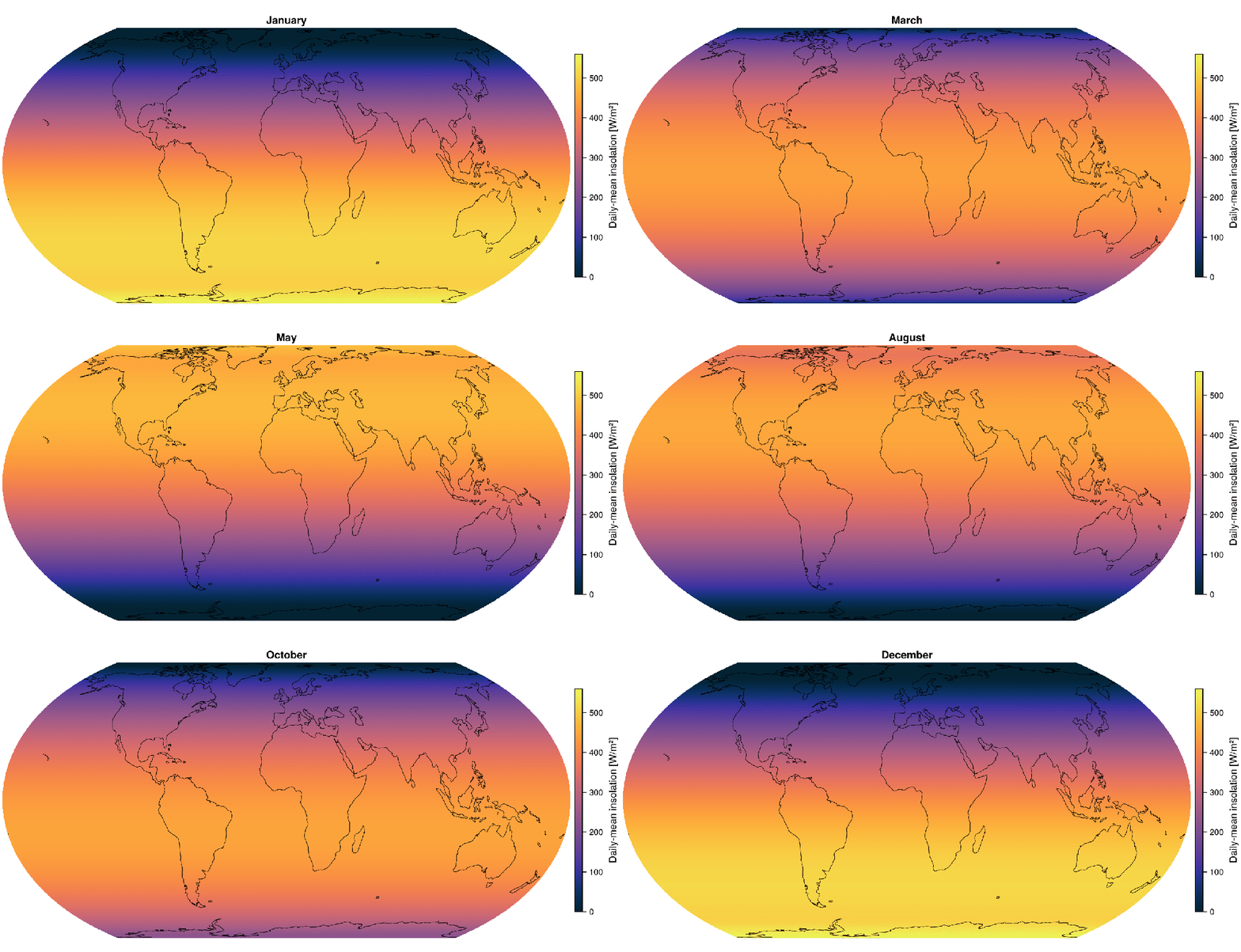
The two most familiar ways we experience insolation are the daily rising and setting of the Sun, and the changing of the seasons. Our lives are paced by the diurnal cycle, but it is the day’s averaged insolation that produces seasonality—and that will be our focus here. In the annual mean, insolation at the top of Earth’s atmosphere is maximal at the equator and decreases toward the poles (right panel below), which will surprise no one. But the magnitude is striking: Earth’s equator receives more than twice the energy of its poles, about 415 versus 171 W/m². Left unchecked, that contrast would produce a far harsher climate than the one we live in. What tempers it is atmospheric and oceanic heat transport, which carries energy poleward and moderates what would otherwise be an enormous temperature contrast between equator and poles.

The surprises begin when you look within the year. At summer solstice, the most sunlit place on Earth is not the subsolar point in the tropics, where the Sun stands directly overhead at midday; it is the pole. The Sun hangs low in the polar sky, but it does not set, and the length-of-day effect wins: integrated over a day, no place on Earth receives more sunlight at the top of the atmosphere than the pole in midsummer. The effect is visible in the left panel above. And the South Pole receives more sunlight in its midsummer than the North Pole does in its own, because right now perihelion—Earth’s closest approach to the Sun—occurs in January.

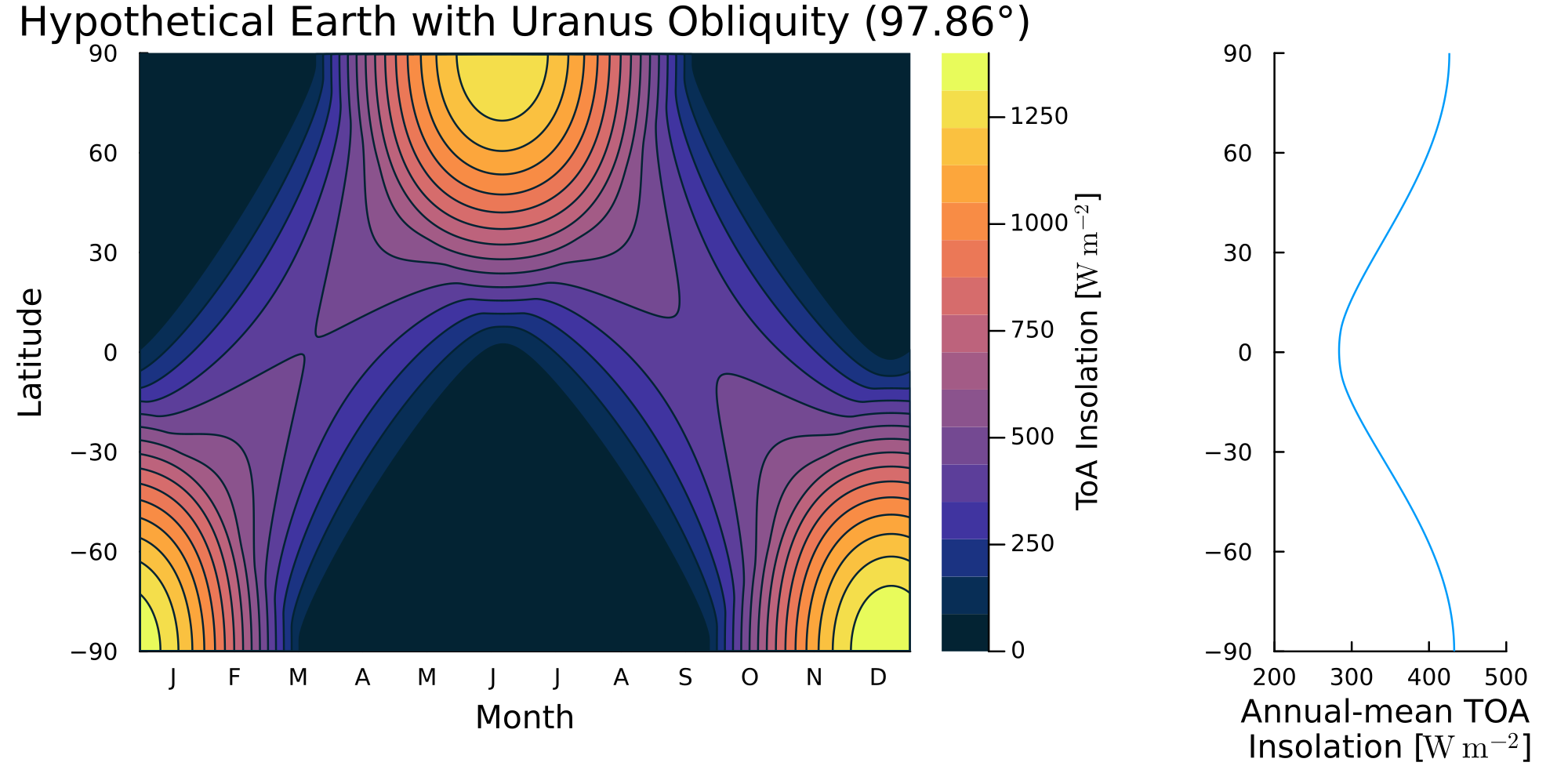
This polar maximum is a consequence of obliquity, the tilt of Earth’s spin axis against the orbital plane, currently 23.4°. It appears whenever the obliquity exceeds about 20.7° (holding the other orbital parameters at Earth’s values). Perhaps more surprising is what happens if the obliquity exceeds about 54°: then the annual-mean insolation becomes maximal at the poles. A planet like that has an equator that is, over the year, the dimmest place on it, and it endures extreme seasons: the summer hemisphere bathed in continuous light, the winter hemisphere dark for months. Uranus, with an obliquity of 98°, orbits the Sun lying on its side and has a seasonal cycle like that; its poles receive more annual sunlight than its equator. With Insolation.jl, we can compute what Earth would experience at such an extreme obliquity (shown below).

Milankovitch cycles and the mystery of the ice ages

Earth’s orbit is not fixed: gravitational tugs from the other planets and torques on Earth’s equatorial bulge make the orbital geometry drift over millennia. The slow changes in three orbital parameters turn out to pace the rise and fall of ice ages. Precession determines at what time of year Earth is closest to the Sun, completing a lap of the calendar once every 21,000 years; obliquity oscillates between 22.1° and 24.5° with a 41,000-year period; and eccentricity, which measures how elliptical Earth’s orbit is, swells and shrinks with periods near 100,000 and 405,000 years. These slow rhythms carry the name of Milutin Milankovitch, and they are written into Earth’s climate record.

The story of how they got there is one of the great detective stories of science. After Louis Agassiz argued in 1840 that erratic boulders and moraines scattered across Europe and North America were left by vanished ice sheets, the question became what made the ice come and go. James Croll proposed in the 1860s that glacials begin when winters are long and cold. Milankovitch, computing by hand through the first half of the 20th century, turned the argument around: what matters is not winter but summer. When summer sunlight at high northern latitudes is weak, winter snow survives the melt season, and ice sheets grow. He calculated how the orbital cycles modulate summer insolation at 65°N and postulated that the ice ages should march to their beat.

He died before the data existed to test the idea. It took until 1976, when Hays, Imbrie, and Shackleton found the orbital periods written into ocean-sediment records: the orbit does pace the ice ages. But the record answers one question and poses others. Obliquity, which merely shifts sunlight between poles and tropics without changing the planetary total, leaves the clearest imprint on global temperature. How does a redistribution become a global signal? Precession, despite its strong effect on peak summer sunlight, is nearly absent from the global temperature record, perhaps because it changes the peak but not the total: a summer near perihelion is brighter but also shorter, since Earth moves faster there, and the two effects cancel in the seasonal sunlight total. And for the past million years, the ice ages have followed a roughly 100,000-year beat whose direct orbital forcing is weak, so the amplitude must come from feedbacks—from ice sheets and the carbon cycle, for example—that remain incompletely understood.

Mysteries like these are part of why we built the CliMA model. A model that aims to predict a warmer future should also be able to explain the climates of the past—they are among the few out-of-distribution tests nature has run for us.

A small package with a long reach

Insolation.jl is one of the smallest packages in the CliMA stack. Computing insolation looks trivial until you need it everywhere: at every grid point and timestep of an atmosphere model, on GPUs, for the diurnal cycle in a weather configuration and the orbital configuration of a paleoclimate run. Insolation.jl provides one implementation, tested against astronomical references, that serves all of these uses. Its orbital parameters—obliquity, eccentricity, longitude of perihelion, and the total solar irradiance—live in ClimaParams.jl, the single source of truth for parameters across the CliMA stack (more on that in a few weeks). Ask for Earth 8,000 years ago and it evaluates the Laskar orbital solution; hand it the parameters of another planet and the same few lines compute the seasons of Mars or a high-obliquity exoplanet. This universality, in miniature, is what we aimed for with all of CliMA.

See for yourself

Reproducing the figure at the top takes a few lines of Julia:

# Install packages by running the following commented line
# using Pkg; Pkg.add(["Insolation", "Plots", "ClimaParams"])

using Insolation, Plots, Dates, Statistics, ClimaParams

params = InsolationParameters(Float64)
od = OrbitalDataSplines()
days, lats = 0:365, -90:90
dates = DateTime(2026, 1, 1) .+ Day.(days)

# compute insolation for each day and latitude pair 
insol_data = daily_insolation.(dates, lats', params, od, false)
F = getproperty.(insol_data, :F) # extract insolation from struct

# now visualize the matrix of insolation values
p1 = contourf(
    days,
    lats,
    F',
    c = :thermal,
    xlabel = "Days since Jan 1, 2026",
    ylabel = "Latitude",
    colorbar_title = "ToA Insolation [W/m2]",
    title = "Modern Earth: Daily-Averaged Insolation",
)
p2 = plot(
    vec(mean(F, dims = 1)), # annual mean insolation by latitude
    lats,
    xlabel = "Annual-mean TOA \nInsolation [W/m2]",
    ylims = (-90, 90),
    yticks = -90:30:90,
    legend = false,
)

plot(
    p1,
    p2,
    layout = grid(1, 2, widths = (0.8, 0.2)),
    size = (900, 450),
    dpi = 300,
    left_margin = 5Plots.mm,
    bottom_margin = 6Plots.mm,
    right_margin = 6Plots.mm,
)

savefig("insolation_example.png")

Change date to a solstice 11,000 years ago, or set the obliquity to 60°, and rerun—you can reproduce the results of the calculations that occupied Milankovitch for decades. A complete runnable tutorial, including the Milankovitch time series, is in the Insolation.jl documentation. For the orbital mechanics behind all of this (Kepler’s laws, the zenith-angle geometry, and the Milankovitch cycles in detail), see chapter 3 of the forthcoming book Physics of Earth’s Climate.

If you find the package useful, a star on the repository helps others discover it.

Insolation.jl was first written by Clare Singer, then a graduate student at Caltech, and is maintained by the CliMA team; the full list of contributors is on GitHub.