
Weather disasters are extremely damaging to humans (e.g., severe storms, heat waves, and flooding), our livelihoods (e.g., drought and wildfire), and to the environment (e.g., coral bleaching via marine heatwaves). Although heavy storms, severe drought, and prolonged heat waves are rare, they account for the majority of the resulting negative impacts. For individuals, governments, and businesses to be able to best prepare for these events, their frequency and severity need to be quantified accurately. A major challenge, however, is that we need to form our estimates using a limited amount of historical data and simulations, where extreme events appear rarely. Moreover, quantifying weather-related risks based on recorded history is already becoming inadequate because climate change is shifting probabilities of rare events; for example, the probability of Hurricane Harvey’s devastating rainfall in Harris County, TX, in 2017 was estimated to have been tripled by recent climate change1. Recorded history will not generalize well to the future, when severe weather events will be both more common and more extreme thanks to climate change.
Quantifying extreme events
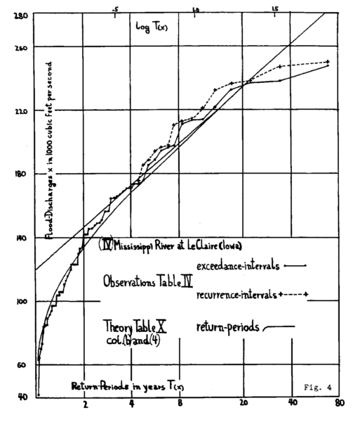
At a minimum, we need an understanding of the probability of events of different magnitudes. A return curve is a graph showing the return period, or typical time between events exceeding a given magnitude, as a function of event magnitude, or severity. An early example of a return curve for water discharge from the Mississippi River is shown in Figure 1. From this one can immediately learn, for example, that discharges of 200,000 cubic feet per second occur about every 8 years. This can then be used in an offline flood model to understand which areas nearby could be inundated.
Computing return curves using parametric statistics
Suppose we have a set of \(N\) observed events of given magnitudes \({a_i}, i \in [1,N]\), collected over a period \(\tau\). For example, this could be a set of observed discharge levels in the past 80 years, as in Figure 1, or a set observed in 80 years of simulations. The probability of observing a return of an event exceeding magnitude \(a\) in time \(\tau\) is given by \(\hat{p}_a = k_a/N\), where \(k_a\) is the observed number of events exceeding \(a\). By assuming that the time between events is exponentially distributed, as in a Poisson process, we can also obtain an estimate for the return period for events exceeding a magnitude \(a\) as
$$r(a) = -\frac{\tau}{\log{(1-\hat{p}_a})} \approx \frac{\tau}{\hat{p}_a},$$
where the approximation holds for very rare events (small \(\hat p_a\) ). Repeating this for different thresholds \(a\) generates the return curve.
A drawback of this approach lies in the uncertainty in our estimates. Assuming that the observed number of events is small compared with \(N\), the relative uncertainty2 in our estimate of the return period \(r(a)\) is
$$\sigma_{r(a)}/r(a) = \sigma_{p_a}/p_a\approx \frac{1}{\sqrt{k_a}}.$$
This is unacceptable for rare events, where \(k_a\) is small, and it breaks down completely for unobserved events, where \(k_a=0\). Generating a larger sample size can be infeasible, even when our “data” comes from simulations with a climate model, as simulating the Earth’s climate for long periods is computationally expensive.
In the above, we assumed a parametric distribution (Poisson) for the time between events in order to estimate a return period. When computing probabilities related to tail events, it turns out that there is a more useful assumption that we can make: that extrema in the data are generated from the generalized extreme value (GEV) distribution3. This helps alleviate the core issue above, because we can infer the (small) set of parameters of this distribution using an existing data set, and then extrapolate using the functional form of the distribution to unseen events. For example, the “theory” curve in Figure 1 is what one would get by fitting the Gumbel distribution to the data: it agrees with the data, but also extends to discharge levels never observed. For further reading, we would direct the reader to the textbook by Stuart Coles.
A digression on importance sampling
The core issue described above is that “events” of any dynamical system have some natural distribution of occurrence. Extreme events correspond to the tail of these distributions, and as a result it can be costly to generate enough examples to compute meaningful statistics. Importance sampling is a method for reducing uncertainty about the probability of these types of events: we instead sample events \(x\) from a distribution (called the importance distribution, which we’ll call \(g(x)\)) where the rare events are common. Accurate statistics for any quantity \(\theta(x)\) under the natural distribution \(f(x)\) are straightforward to compute by taking into account the likelihood ratio \(f(x)/g(x)\), because \(\int \theta(x) f(x) dx = \int \theta(x) (f(x)/g(x)) g(x) dx\). Moreover, by choosing a good importance distribution, the variance in the estimators can be greatly reduced4 compared with the simple approach outlined above.
As a simple example, consider trying to estimate the probability of events \(x > 5\) based on a finite sample of data \(\{x\}\) drawn from a zero mean unit variance Gaussian, i.e., \(x \sim f(x) = N(0, 1)\). The true probability of this event can be calculated analytically as approximately \(p = \int_{5}^\infty f(x) dx \approx 3 \times 10^{-7}\). By our above calculation, if we want a relative error \(\sigma_p/p \approx\)10% in this estimate, we would need to sample 300 million times! If we instead draw 500 samples from the importance distribution \(x \sim g(x) = N(5,1)\), and compute the probability as
$$\hat{p} = \frac{1}{500}\sum_{j=1}^{500} \mathscr{H}(x_j-5) \frac{f(x_j)}{g(x_j)}$$
(where \(\mathscr{H}\) is the Heaviside function), we obtain an estimate for \(p\) with our desired relative error of 10% (estimated in this case with bootstrapping). The usability of this approach hinges on being able to (1) efficiently generate samples from the importance distribution and (2) compute the likelihood ratio easily. We will now describe another method for estimating the probability of rare events, in which the samples from the importance distribution are trajectories of a dynamical system which exhibit rare behavior.
Computing return curves using ensembles of trajectories: the GKLT algorithm
The Giardina-Kurchan-Lecomte-Tailleur (GKLT) algorithm is a method for generating samples from an implicit importance distribution. With the GKLT algorithm, an ensemble (of hundreds to thousands) of trajectories are evolved forward in time concurrently. Periodically, these trajectories are scored according to a case-specific metric which identifies those exhibiting “extreme” behavior – for example, spatially averaged temperatures exceeding some threshold. Trajectories that are more extreme have a higher probability of being cloned, while those that are not are more likely to be cut. The updated trajectory set is then evolved forward in time until the next clone/cut time. Under certain conditions (on the clone/cut time, on the metric used to score the trajectories, and on the ensemble size), this process converges such that the final set of trajectories are samples from an implicit importance distribution, under which the “typical” trajectories exhibit extreme behavior according to the metric chosen. Crucially, the likelihood ratio relative to the natural distribution is computable, and so the ensemble can be used to compute statistics, like return curves, under the natural distribution, as described above.
An example of the results of this algorithm is shown in Figure 2, for the 1-d Ornstein-Uhlenbeck stochastic process. For the same computational cost as a direct numerical integration, the GKLT algorithm produces a return curve to approximately 1,000x longer return times. The GEV distribution was also fit to the direct simulation data; it can extrapolate to any return period, but has large uncertainties if the data used to fit the parameters is not sufficient5.
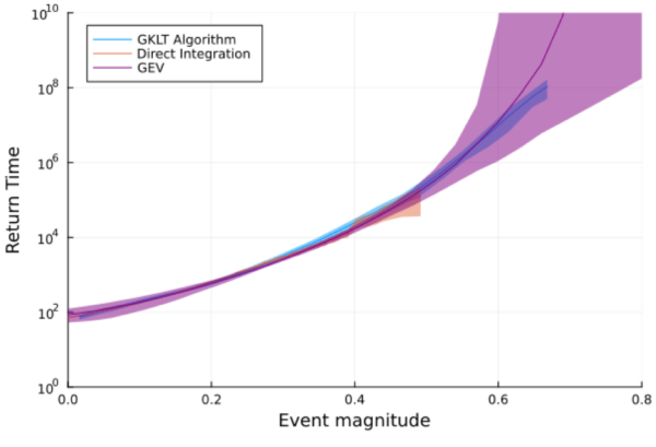
In this particular example, it would have been possible to compute longer return periods using direct simulations because the computational cost of simulating the Ornstein-Uhlenbeck process is relatively low. The same is not true for more complex dynamical systems like the Earth’s climate. The GKLT algorithm has been applied successfully for computing return curves of heat waves using realistic climate simulations, including with CESM. A key additional benefit of this algorithm is the resulting trajectory ensemble, which can be used to study the physics of extreme events, including spatially and temporally correlated extremes in temperature6. These trajectories can also be used to augment training data of machine learning algorithms with the goal of improving generalizability. A possible drawback of the method is that the ensemble has been tailored to a specific type of extreme via the chosen metric; different extremes under study would in principle require separate ensemble runs. This method can also only be applied to numerical simulations, and not to historical data.
Applications and further reading
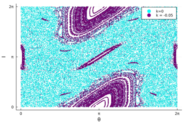
A quick literature search will pull up many interesting applications of GEV and importance sampling methods for rare events (GKLT and genealogical particle analysis), from machine learning to solar system dynamics. A review of large deviation theory and applications to climate can be found here. As mentioned, other extremes can be considered: in a very neat application, the GKLT algorithm can be used to sample a distribution centered on orbits with with rare values of the (finite time) estimate of the maximum Lyapunov exponent. In Figure 3, we show a figure recreated from the original GKLT paper, showing how the algorithm can be used to select regular orbits of the standard map, in spite of the fact that most orbits for this system are chaotic for this parameter choice.
We would like to apply these tools to simulations of the Earth’s climate made using the CliMA Earth System Model. Provided that our model can accurately simulate the future climate under different climate change scenarios, we will then be able to start to address the problem of quantifying extreme events in a warming world.
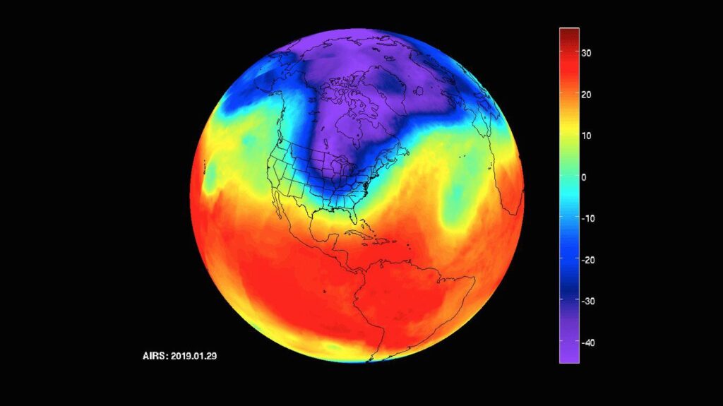
Feature image courtesy NASA/JPL-Caltech. An image of a polar vortex, which caused surface temperatures as low as -40F and wind chill as low as -50F, captured by NASA’s AIRS instrument, from 2019.
1See K. Emanuel, 2017, M. D. Risser and M. F. Wehner, 2017, and Van Oldenborgh et al., 2017.
2See, e.g., Carney et al. 2020 or a statistics textbook for a more thorough derivation.
3More specifically, that the distribution of extrema taken over blocks of data limits to the GEV distribution as the block length grows.
4See, e.g., https://www.math.arizona.edu/~tgk/mc/book_chap6.pdf.
5We refer the reader again to Carney et al. 2020 for a comparison of rare event probability estimate methods.
6These trajectories are close to true trajectories of the system (despite small perturbations at each clone step, via the Shadowing Theorem).