
By Eviatar Bach and Oliver Dunbar
To understand this blog post, you will need some basic familiarity with probability (Bayes’ theorem, covariance) and multivariate calculus.
In climate modeling, small-scale processes that cannot be resolved, such as convection and cloud physics, are represented using parameterizations (see two previous blog posts here and here). The parameterizations depend on uncertain parameters, which leads to uncertainty in simulations of future climates. At CliMA, we use observations of the current climate, as well as high-resolution simulations, to estimate these parameters. The learning problem is challenging, as the parameterized processes typically are not directly observable, and the data itself has a low signal-to-noise ratio due to the chaotic nature of the Earth system. To deal with these challenges, we apply ensemble Kalman inversion, and its variants, to accumulated climate statistics to arrive at estimates of the parameters.
Ensemble Kalman inversion was first introduced by Iglesias et al. (2013) as a method to solve inverse problems and has since been extended and applied to a variety of problems. Here we give a basic introduction to the method, as well as an example using the EnsembleKalmanProcesses.jl library developed at CliMA.
Formulation of an inverse problem
Let the parameters of a model be denoted by a vector \(\theta\). We assume that there are true values of these parameters that reflect the real-world physics, and we denote them by \(\theta^*\). The data, coming from observations or high-resolution simulations, are denoted \(y\). The forward map \(\mathscr{G}\) is a function that takes as input the parameters \(\theta\) and maps them to the space of observations. In particular, we assume that \(y\) arises through an evaluation of \(\mathscr{G}\) at the true parameters, with additive observational noise \(\eta\):
\[y = \mathscr{G}(\theta^*) + \eta.\]
Though we do not know a priori the value of \(\theta^*\), we assume that we have some prior knowledge about \(\theta\), such as the range of likely or physically reasonable values. The forward map \(\mathscr{G}\) typically involves a composition of three maps: parameter transformation, climate model evaluation, and data processing (e.g., accumulation of statistics and dimension reduction). Data is typically time-averaged rather than instantaneous, so that the forward map can be treated independently of initial conditions.
The task of the Bayesian inverse problem is the following: using \(y\) and the prior distribution of \(\theta\), find the posterior distribution \(\theta \mid y\), which is the conditional probability of the parameter values given the data. Often, we cannot obtain the full posterior, but we can obtain useful statistics such as its mode (maximum a posteriori, or MAP, estimation) or covariance. Kalman methods take advantage of Gaussian assumptions to simplify the inference problem.
The linear inverse problem
We begin with a simple but illustrative setting: a linear inverse problem where \(\mathscr{G}(\theta) = G\theta\), so that
\[y = G\theta + \eta,\]
where \(\eta\sim\mathscr{N}(0, \Gamma)\). Suppose that we have prior knowledge about \(\theta\), namely, that it comes from the distribution \(\theta\sim\mathscr{N}(\theta_0, C^{\theta\theta})\).
By Bayes’ rule,
\[p(\theta|y) \propto p(y|\theta)p(\theta).\]
We have that \(y|\theta\sim\mathscr{N}(G\theta, \Gamma)\). Substituting the expressions for the multivariate normal,
\[\begin{aligned}p(\theta|y)&\propto \exp\left(-\frac{1}{2}(y – G\theta)^T\Gamma^{-1}(y – G\theta)\right)\\&\qquad\times\exp\left(-\frac{1}{2}(\theta – \theta_0)^T(C^{\theta\theta})^{-1}(\theta – \theta_0)\right)\\&= \exp\!\Big(\!-\frac{1}{2}(y – G\theta)^T\Gamma^{-1}(y – G\theta)\\&\qquad\qquad- \frac{1}{2}(\theta – \theta_0)^T(C^{\theta\theta})^{-1}(\theta – \theta_0)\Big).\end{aligned}\]
We now seek the value of \(\theta\) that corresponds to the mode of the posterior, that is, the value of \(\theta\) that maximizes \(p(\theta|y)\), which we will call \(\hat{\theta}\). This is equivalent to finding a minimizer of the negative log-likelihood \(-\log p(\theta|y)\):
\[\begin{aligned}
\hat{\theta} &= \arg\min [-\log p(\theta|y)]\\
&= \arg\min\left[\frac{1}{2}(y – G\theta)^T\Gamma^{-1}(y – G\theta) + \frac{1}{2}(\theta – \theta_0)^T(C^{\theta\theta})^{-1}(\theta – \theta_0)\right].\end{aligned}\]
To minimize this, we take the derivative and set it to zero. We make use of matrix calculus to do this:
\[\frac{d(-\log p(\theta|y))}{d\theta}\Big|_{\theta=\hat{\theta}} = (C^{\theta\theta})^{-1}(\hat{\theta} – \theta_0) – G^T\Gamma^{-1}(y – G\hat{\theta}) = 0.\]
Taking a second derivative, we can verify this is a minimum. Because covariance matrices (and therefore their inverses) are positive definite,
\[(C^{\theta\theta})^{-1} + G^T\Gamma^{-1} G > 0.\]
Solving for \(\hat{\theta}\), we obtain
\[\hat{\theta} = \theta_0 + C^{\theta\theta} G^T(\Gamma + GC^{\theta\theta}G^T)^{-1}(y – G\theta_0) = \theta_0 + K(y- G\theta_0),\]
where \(K\equiv C^{\theta\theta} G^T(\Gamma + GC^{\theta\theta}G^T)^{-1}\) is often called the Kalman gain. Thus, we can write
\[\hat{\theta} = \theta_0 + K(y – G\theta_0).\]
In the linear case, this is the optimal estimate (i.e., the MAP estimator) and we are done. In the nonlinear case, we must do something different.
The nonlinear inverse problem
We will now make a formal substitution of a linear forward model with a nonlinear one in the Kalman update.
We first rewrite the Kalman gain from the linear case in a new notation
\[K \equiv C^{\theta G} (\Gamma + C^{GG})^{-1},\]
where \(C^{\theta G} \equiv \mathbb{E}[(\theta – \mathbb{E}[\theta])(G\theta – \mathbb{E}[G\theta])^T]\) is the cross-covariance between \(\theta\) and \(G\theta\) and \(C^{GG} \equiv \mathbb{E}[(G\theta – \mathbb{E}[G\theta])(G\theta – \mathbb{E}[G\theta])^T]\) is the covariance of \(G\theta\).
Now, if \(G\) is nonlinear, which we write as \(\mathscr{G}(\theta)\), we substitute the nonlinear model for the linear one in the covariance matrices, i.e.,
\[C^{\theta \mathscr{G}}=\mathbb{E}[(\theta – \mathbb{E}[\theta])(\mathscr{G}(\theta) – \mathbb{E}[\mathscr{G}(\theta)])^T]\] and \[C^{\mathscr{G} \mathscr{G}}=\mathbb{E}[(\mathscr{G}(\theta) – \mathbb{E}[\mathscr{G}(\theta)])(\mathscr{G}(\theta) – \mathbb{E}[\mathscr{G}(\theta)])^T].\]
A Gaussian prior becomes a Gaussian posterior under a linear transformation, so in the linear case this representation is exact. In the nonlinear case, a Gaussian prior will not yield a Gaussian posterior, and so there is no hope of recovering higher order information (e.g. skew) with this algorithm. However, in practice this substitution often works well to recover an approximation of the MAP. The update using \(K\) does not involve taking any derivatives of \(\mathscr{G}(\theta)\) with respect to \(\theta\), and in practice this flexibility is particularly useful.
Ensemble Kalman inversion
It is often intractable to compute \(C^{\theta\mathscr{G}}\) and \(C^{\mathscr{G}\mathscr{G}}\). A remarkably effective way of approximating these matrices is by introducing an ensemble, that is, we work directly with a finite set of samples from the distribution of \(\theta\). In this way, we can replace \(C^{\theta\mathscr{G}}\) and \(C^{\mathscr{G}\mathscr{G}}\) by their empirical approximations from this sample:
\[C^{\theta \mathscr{G}}=\frac{1}{J}\sum_{j=1}^J[(\theta^{(j)} – \overline{\theta})(\mathscr{G}(\theta^{(j)}) – \overline{\mathscr{G}(\theta)})^T]\]
\[C^{\mathscr{G} \mathscr{G}}=\frac{1}{J}\sum_{j=1}^J[(\mathscr{G}(\theta^{(j)}) – \overline{\mathscr{G}(\theta)})(\mathscr{G}(\theta^{(j)}) – \overline{\mathscr{G}(\theta)})^T]\]
We use overbar notation to represent taking the mean over the ensemble, and we arrive at the following update for each member of the ensemble
\[\hat{\theta}^{(j)} = \theta^{(j)} + C^{\theta\mathscr{G}}(\Gamma + C^{\mathscr{G}\mathscr{G}})^{-1}(y – \mathscr{G}(\theta^{(j)})).\]
With large ensemble size, in the linear problem we (effectively) reach the optimum in one step. In the nonlinear case, however, we may have to do multiple iterations, taking the posterior of the last iteration as the prior for the next iteration. Though there are no derivatives of \(\mathscr{G}(\theta)\) with respect to \(\theta\), this iterative procedure is still related to performing gradient descent on the cost function introduced earlier; see Calvello et al. (2022) for more details.
To summarize, the algorithm is as follows:
- Draw J samples from the prior distribution on the parameters, \(\theta_0^{(j)}\sim \mathscr{N}(\theta_0, C^{\theta\theta}), j=1,\ldots,J\).
- Now repeat the following steps for iterations \(i=1,\ldots,N\):
a. Run the forward model \(\mathscr{G}\) with each \(\theta_i^{(j)}\), obtaining \(\mathscr{G}(\theta_i^{(1)}),\ldots,\mathscr{G}(\theta_i^{(J)})\).
b. Compute the empirical covariances \(C_i^{\theta\mathscr{G}}\) and \(C_i^{\mathscr{G}\mathscr{G}}\) using the samples.
c. Obtain the next ensemble by computing \(\theta_{i+1}^{(j)} = \theta_i^{(j)} + C_i^{\theta\mathscr{G}}(\Gamma + C_i^{\mathscr{G}\mathscr{G}})^{-1}(y – \mathscr{G}(\theta_i^{(j)}))\).
- \(\overline{\theta}_N\) will now be the best estimate of the parameters solving the inverse problem.
One might hope that taking empirical covariance of the ensemble after some number of iterations also provides a good estimate of the parameter uncertainty, but unfortunately this is not the case. We have three ways around this, (i) adaptive learning rates can terminate the algorithm nearer to a Gaussian estimate of the spread (ii) the ensemble Kalman sampler algorithm which also aims to provide a better Gaussian estimate of the spread; and (iii) the calibrate–emulate–sample procedure that uses the EKI ensemble to train a machine learning surrogate for sampling the posterior distribution.
Unscented Kalman inversion
Unscented Kalman inversion (UKI) was introduced by Huang et al. (2022) as a variant of EKI. Here, given the mean and covariance at iteration \(i\), a set of sigma points are chosen that have this mean and covariance. In comparison, EKI samples are not taken at fixed points. Then, for the next iteration these sigma points are evaluated using the forward model, as in step 2a of EKI, and these forward model evaluations are further used to estimate \(C^{\theta\mathscr{G}}\) and \(C^{\mathscr{G}\mathscr{G}}\) in the Kalman gain. The sigma points are designed to accurately approximate the impact of the forward model on the mean and covariance compared to random samples, and expressions for them are given in Eq. 20 of Huang et al. (2022).
UKI is sometimes observed to have better performance than EKI for challenging inverse problems, though at the cost of more tunable algorithmic parameters. EnsembleKalmanProcesses.jl includes implementations of both EKI and UKI, as well as several other variants.
An Example with code
We now provide an example of applying ensemble Kalman inversion to a simple problem, using the EnsembleKalmanProcesses.jl package in the Julia language.
In this example we have a model that produces a sinusoid \(f(A,v)=A \sin(\phi+t)+v,\forall t\in [0,2\pi]\), with a random phase \(\phi\). Given an initial guess of the parameters as \(A\sim \mathscr{N}(2,1)\) and \(v\sim\mathscr{N}(0,25)\), our goal is to estimate the parameters from a noisy observation of the maximum, minimum, and mean of the true model output.
First, we load the packages we need:
using LinearAlgebra, Random

using Distributions, Plots

using EnsembleKalmanProcesses
using EnsembleKalmanProcesses.ParameterDistributions
const EKP = EnsembleKalmanProcesses
Now, we define a model which generates a sinusoid given parameters \(\theta\): an amplitude and a vertical shift. We will estimate these parameters from data. The model adds a random phase shift upon evaluation.
dt = 0.01
trange = 0:dt:(2 * pi + dt)
function model(amplitude, vert_shift)
    phi = 2 * pi * rand()
    return amplitude * sin.(trange .+ phi) .+ vert_shift
end
We then define \(\mathscr{G}(\theta)\), which returns the observables of the sinusoid given a parameter vector. These observables should be defined such that they are informative about the parameters we wish to estimate. Here, the two observables are the vertical range of the curve (which is informative about its amplitude), as well as its mean (which is informative about its vertical shift).
function G(theta)
    A, vert_shift = theta
    sincurve = model(A, vert_shift)
    return [maximum(sincurve) - minimum(sincurve), mean(sincurve)]
end
Suppose we have a noisy observation of the true system. Here, we create a pseudo-observation \(y\) by running our model with the correct parameters and adding Gaussian noise to the output.
dim_output = 2

Γ = 0.1 * I
noise_dist = MvNormal(zeros(dim_output), Γ)

theta_true = [1.0, 7.0]
y = G(theta_true) .+ rand(noise_dist)
We now define prior distributions on the two parameters. For the amplitude, we define a prior with mean 2 and standard deviation 1. It is additionally constrained to be nonnegative. For the vertical shift we define a Gaussian prior with mean 0 and standard deviation 5.
prior_u1 = constrained_gaussian("amplitude", 2, 1, 0, Inf)
prior_u2 = constrained_gaussian("vert_shift", 0, 5, -Inf, Inf)
prior = combine_distributions([prior_u1, prior_u2])
We now generate the initial ensemble and set up the ensemble Kalman inversion.
N_ensemble = 5
N_iterations = 5

initial_ensemble = EKP.construct_initial_ensemble(prior, N_ensemble)

ensemble_kalman_process = EKP.EnsembleKalmanProcess(initial_ensemble, y, Γ, Inversion())
We are now ready to carry out the inversion. At each iteration, we get the ensemble from the last iteration, apply \(\mathscr{G}(\theta)\) to each ensemble member, and apply the Kalman update to the ensemble.
for i in 1:N_iterations
    params_i = get_ϕ_final(prior, ensemble_kalman_process)

    G_ens = hcat([G(params_i[:, i]) for i in 1:N_ensemble]...)

    EKP.update_ensemble!(ensemble_kalman_process, G_ens)
end
Finally, we get the ensemble after the last iteration. This provides our estimate of the parameters.
final_ensemble = get_ϕ_final(prior, ensemble_kalman_process)
To visualize the success of the inversion, we plot model with the true parameters, the initial ensemble, and the final ensemble.
plot(trange, model(theta_true...), c = :black, label = "Truth", legend = :bottomright, linewidth = 2)
plot!(
    trange,
    [model(get_ϕ(prior, ensemble_kalman_process, 1)[:, i]...) for i in 1:N_ensemble],
    c = :red,
    label = ["Initial ensemble" "" "" "" ""],
)
plot!(trange, [model(final_ensemble[:, i]...) for i in 1:N_ensemble], c = :blue, label = ["Final ensemble" "" "" "" ""])

xlabel!("Time")
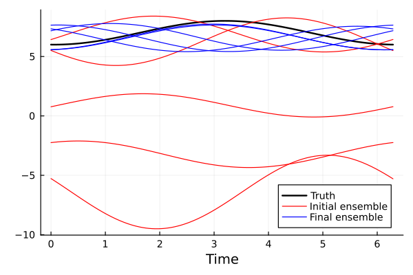
We see that the final ensemble is much closer to the truth. Note that the random phase shift is of no consequence.